Tutorial 2: Using CAP#
![]()
The CAP class is designed to perform CAPs analyses (on all subjects or group of subjects). It offers the flexibility
to analyze data from all subjects or focus on specific groups, compute CAP-specific metrics, and generate visualizations
to aid in the interpretation of results.
Performing CAPs on All Subjects#
All information pertaining to CAPs (k-means models, activation vectors/cluster centroids, etc) are stored as attributes
in the CAP class and this information is used by all methods in the class. These attributes are accessible via
properties.
Some properties can also be used as setters.
import numpy as np
from neurocaps.analysis import CAP
# Extracting timseries
parcel_approach = {"Schaefer": {"n_rois": 100, "yeo_networks": 7, "resolution_mm": 2}}
# Simulate data for example
subject_timeseries = {str(x): {f"run-{y}": np.random.rand(100, 100) for y in range(1, 4)} for x in range(1, 11)}
# Initialize CAP class
cap_analysis = CAP(parcel_approach=parcel_approach)
# Get CAPs
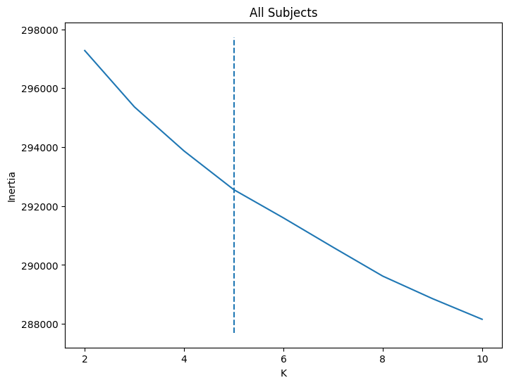
cap_analysis.get_caps(
subject_timeseries=subject_timeseries,
n_clusters=range(2, 11),
cluster_selection_method="elbow",
show_figs=True,
step=2,
progress_bar=True, # Available in versions >= 0.21.5
)
Concatenating Subjects [GROUP: A]: 100%|█████████████████████████████████████████████████████████████████████████████████████████████████████████████████████████████████████| 10/10 [00:01<00:00, 668.15it/s]
Clustering [GROUP: All Subjects]: 100%|████████████████████████████████████████████████████████████████████████████████████████████████████████████████████████████| 9/9 [00:00<00:00, 20.38it/s]
2025-04-07 18:15:07,367 neurocaps.analysis.cap [INFO] [GROUP: All Subjects | METHOD: elbow] Optimal cluster size is 5.
print can be used to return a string representation of the CAP class.
print(cap_analysis)
Metadata:
================================================
Parcellation Approach                           : Schaefer
Groups                                          : All Subjects
Number of Clusters                              : [2, 3, 4, 5, 6, 7, 8, 9, 10]
Cluster Selection Method                        : elbow
Optimal Number of Clusters                      : {'All Subjects': np.int64(5)}
CPU Cores Used for Clustering (Multiprocessing) : None
User-Specified Runs IDs Used for Clustering     : None
Concatenated Timeseries Bytes                   : 2400184 bytes
Standardized Concatenated Timeseries            : True
Co-Activation Patterns (CAPs)                   : {'All Subjects': 5}
Variance Explained by Clustering                : {'All Subjects': np.float64(0.02448526803307005)}
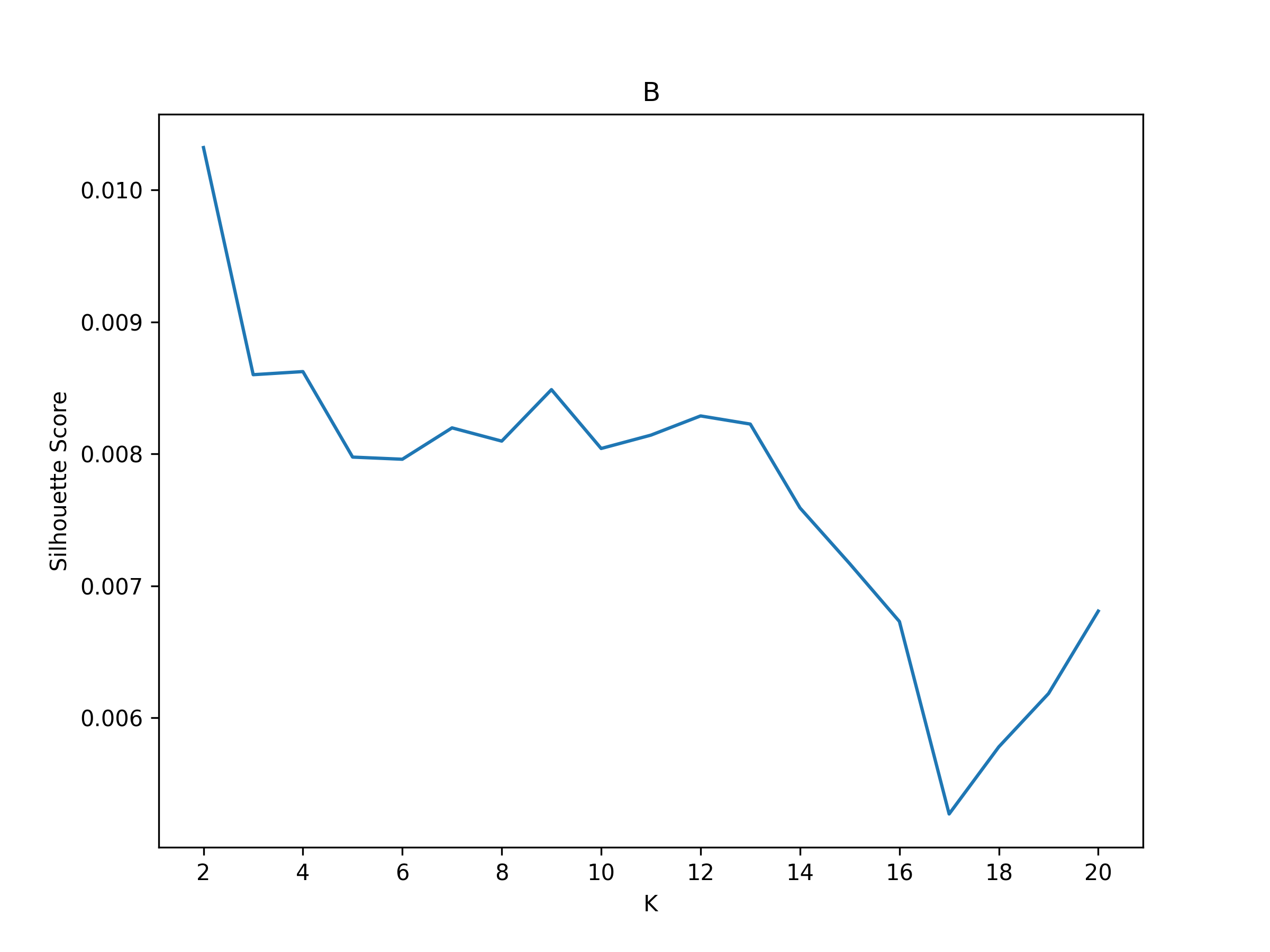
Performing CAPs on Groups#
cap_analysis = CAP(groups={"A": ["1", "2", "3", "5"], "B": ["4", "6", "7", "8", "9", "10"]})
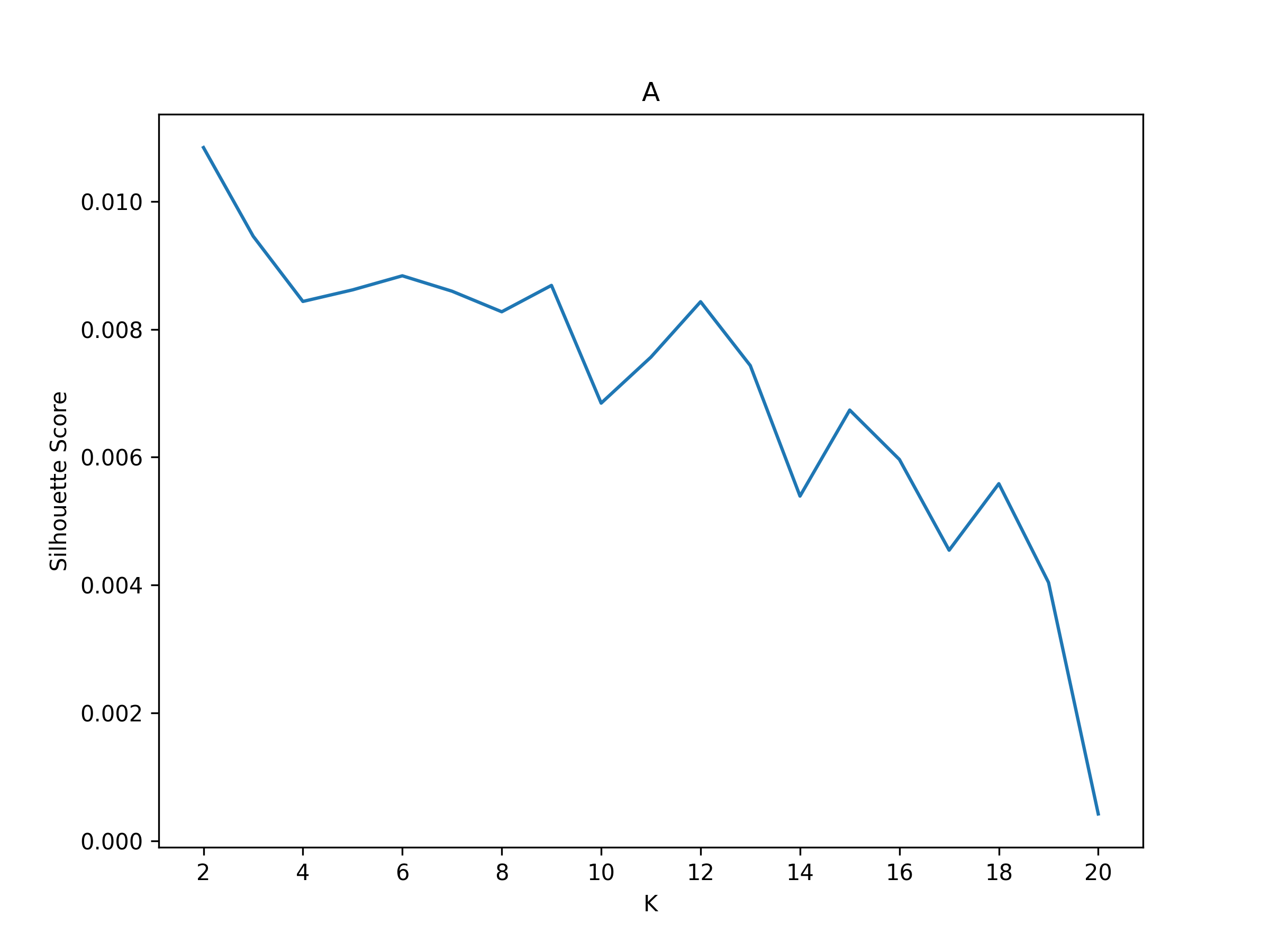
cap_analysis.get_caps(
subject_timeseries=subject_timeseries,
n_clusters=range(2, 21),
cluster_selection_method="silhouette",
show_figs=True,
step=2,
progress_bar=True,
)
Concatenating Subjects [GROUP: A]: 100%|█████████████████████████████████████████████████████████████████████████████████████████████████████████████████████████████████████| 4/4 [00:01<00:00, 582.04it/s]
Concatenating Subjects [GROUP: A]: 100%|█████████████████████████████████████████████████████████████████████████████████████████████████████████████████████████████████████| 6/6 [00:01<00:00, 706.37it/s]
Clustering [GROUP: A]: 100%|█████████████████████████████████████████████████████████████████████████████████████████████████████████████████████████████████████| 19/19 [00:01<00:00, 18.71it/s]
2025-04-07 18:15:53,981 neurocaps.analysis.cap [INFO] [GROUP: A | METHOD: silhouette] Optimal cluster size is 2.
Clustering [GROUP: B]: 100%|█████████████████████████████████████████████████████████████████████████████████████████████████████████████████████████████████████| 19/19 [00:01<00:00, 12.48it/s]
2025-04-07 18:15:55,236 neurocaps.analysis.cap [INFO] [GROUP: B | METHOD: silhouette] Optimal cluster size is 2.
Calculate Metrics#
Note that if standardize was set to True in CAP.get_caps(), then the column (ROI) means and standard deviations
computed from the concatenated data used to obtain the CAPs are also used to standardize each subject in the timeseries
data inputted into CAP.calculate_metrics(). This ensures proper CAP assignments for each subjects frames.
df_dict = cap_analysis.calculate_metrics(
    subject_timeseries=subject_timeseries,
    return_df=True,
    metrics=["temporal_fraction", "counts", "transition_probability"],
    continuous_runs=True,
    progress_bar=True,
)

print(df_dict["temporal_fraction"])
Computing Metrics for Subjects: 100%|███████████████████████████████████████████████████████████████████████████████████████████████████████████████████████████| 10/10 [00:00<00:00, 159.78it/s]
Subject_ID |
Group |
Run |
CAP-1 |
CAP-2 |
|---|---|---|---|---|
1 |
A |
run-continuous |
0.5066666666666667 |
0.49333333333333335 |
2 |
A |
run-continuous |
0.5333333333333333 |
0.4666666666666667 |
3 |
A |
run-continuous |
0.6 |
0.4 |
5 |
A |
run-continuous |
0.54 |
0.46 |
4 |
B |
run-continuous |
0.41333333333333333 |
0.5866666666666667 |
6 |
B |
run-continuous |
0.47333333333333333 |
0.5266666666666666 |
7 |
B |
run-continuous |
0.44 |
0.56 |
8 |
B |
run-continuous |
0.5 |
0.5 |
9 |
B |
run-continuous |
0.4866666666666667 |
0.5133333333333333 |
10 |
B |
run-continuous |
0.46 |
0.54 |
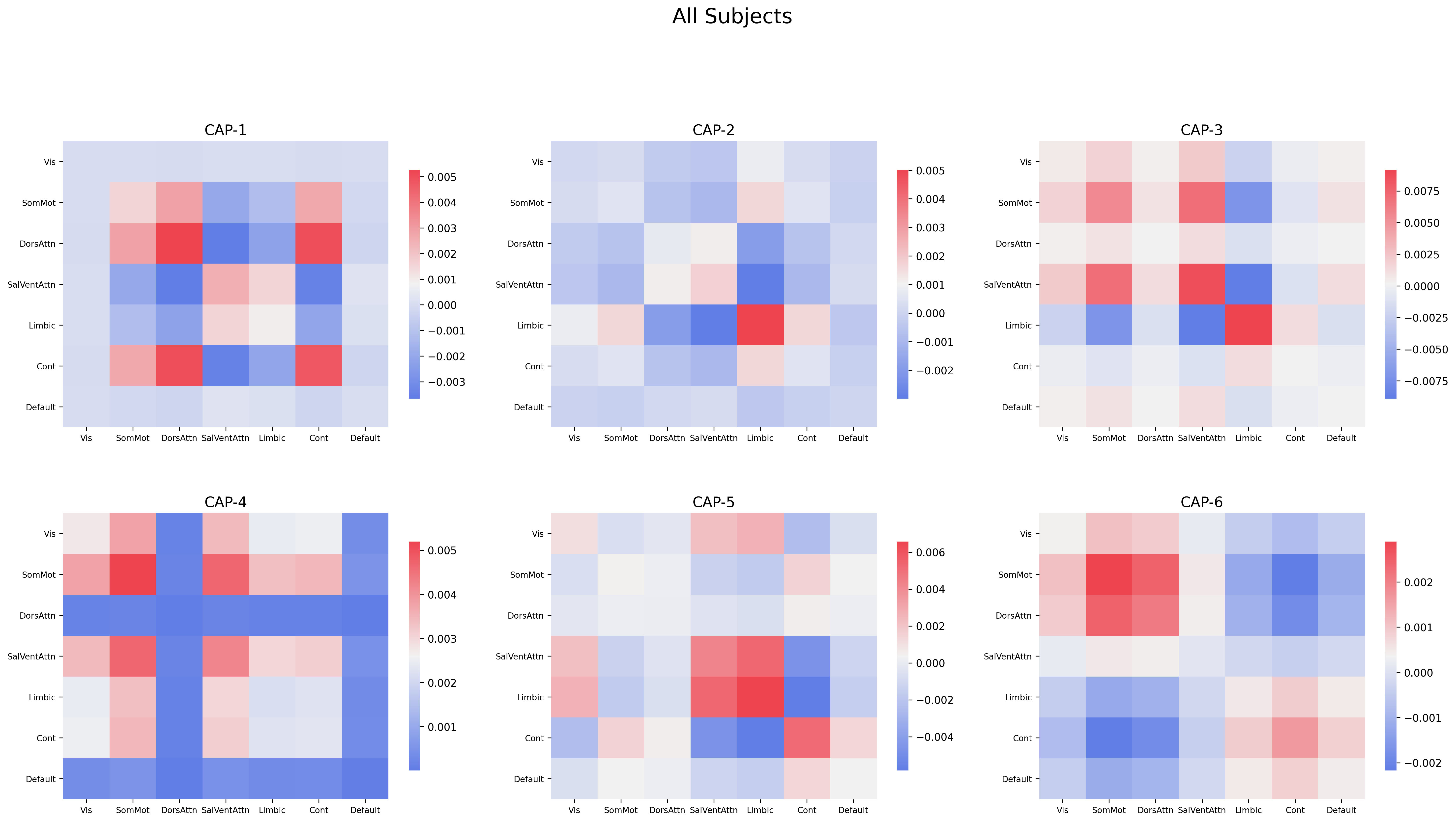
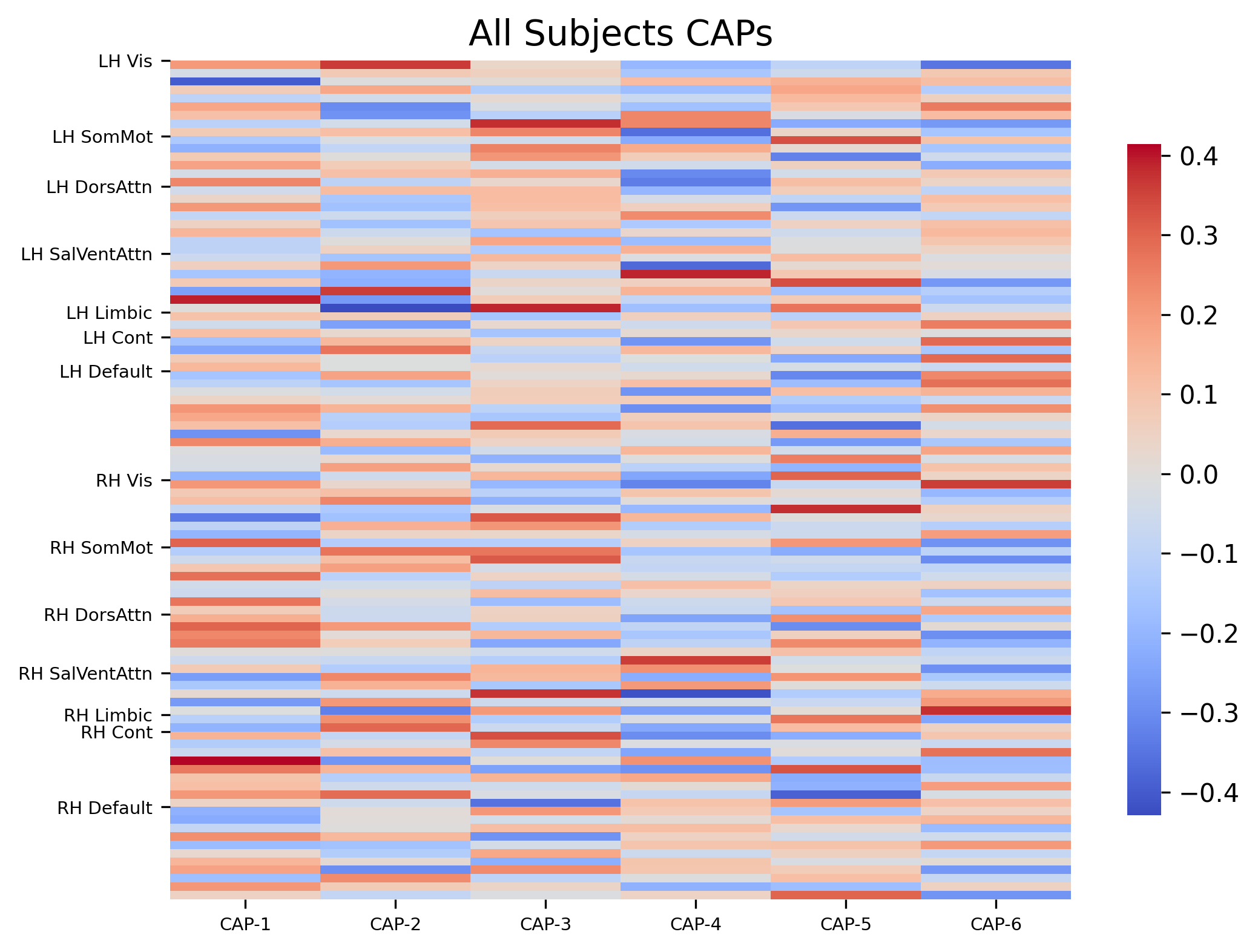
Plotting CAPs#
import seaborn as sns

cap_analysis = CAP(parcel_approach={"Schaefer": {"n_rois": 100, "yeo_networks": 7, "resolution_mm": 1}})

cap_analysis.get_caps(subject_timeseries=subject_timeseries, n_clusters=6)

sns.diverging_palette(145, 300, s=60, as_cmap=True)

palette = sns.diverging_palette(260, 10, s=80, l=55, n=256, as_cmap=True)

kwargs = {
    "subplots": True,
    "fontsize": 14,
    "ncol": 3,
    "sharey": True,
    "tight_layout": False,
    "xlabel_rotation": 0,
    "hspace": 0.3,
    "cmap": palette,
}

cap_analysis.caps2plot(visual_scope="regions", plot_options="outer_product", show_figs=True, **kwargs)
cap_analysis.caps2plot(
    visual_scope="nodes", plot_options="heatmap", xticklabels_size=7, yticklabels_size=7, show_figs=True
)
Generate Pearson Correlation Matrix#
cap_analysis.caps2corr(annot=True, cmap="viridis", show_figs=True)
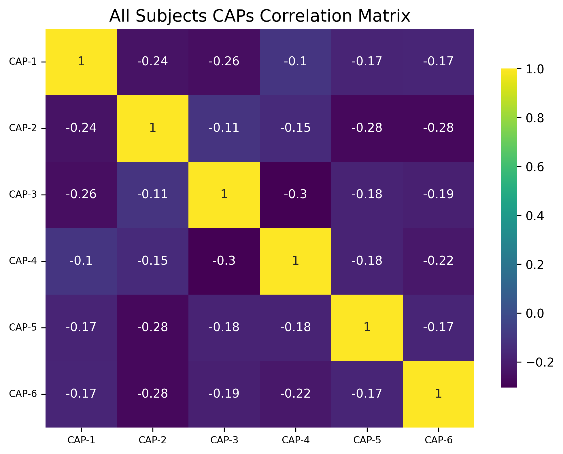
corr_dict = cap_analysis.caps2corr(return_df=True)
print(corr_dict["All Subjects"])
CAP-1 |
CAP-2 |
CAP-3 |
CAP-4 |
CAP-5 |
CAP-6 |
|
|---|---|---|---|---|---|---|
CAP-1 |
1 (0)*** |
-0.24 (0.016)* |
-0.26 (0.01)* |
-0.1 (0.3) |
-0.17 (0.087) |
-0.17 (0.09) |
CAP-2 |
-0.24 (0.016)* |
1 (0)*** |
-0.11 (0.28) |
-0.15 (0.14) |
-0.28 (0.0051)** |
-0.28 (0.0055)** |
CAP-3 |
-0.26 (0.01)* |
-0.11 (0.28) |
1 (0)*** |
-0.3 (0.0021)** |
-0.18 (0.075) |
-0.19 (0.058) |
CAP-4 |
-0.1 (0.3) |
-0.15 (0.14) |
-0.3 (0.0021)** |
1 (0)*** |
-0.18 (0.076) |
-0.22 (0.028)* |
CAP-5 |
-0.17 (0.087) |
-0.28 (0.0051)** |
-0.18 (0.075) |
-0.18 (0.076) |
1 (0)*** |
-0.17 (0.089) |
CAP-6 |
-0.17 (0.09) |
-0.28 (0.0055)** |
-0.19 (0.058) |
-0.22 (0.028)* |
-0.17 (0.089) |
1 (0)*** |
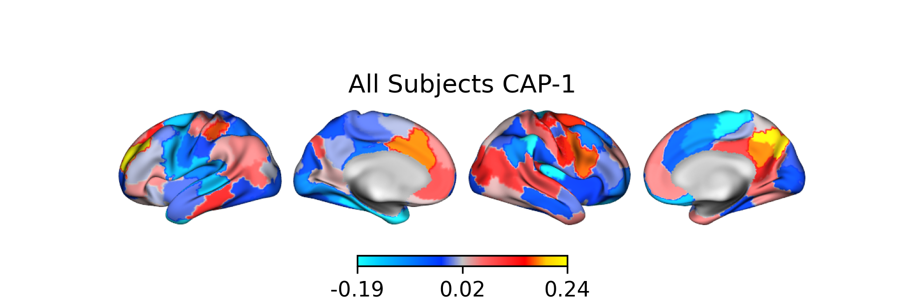
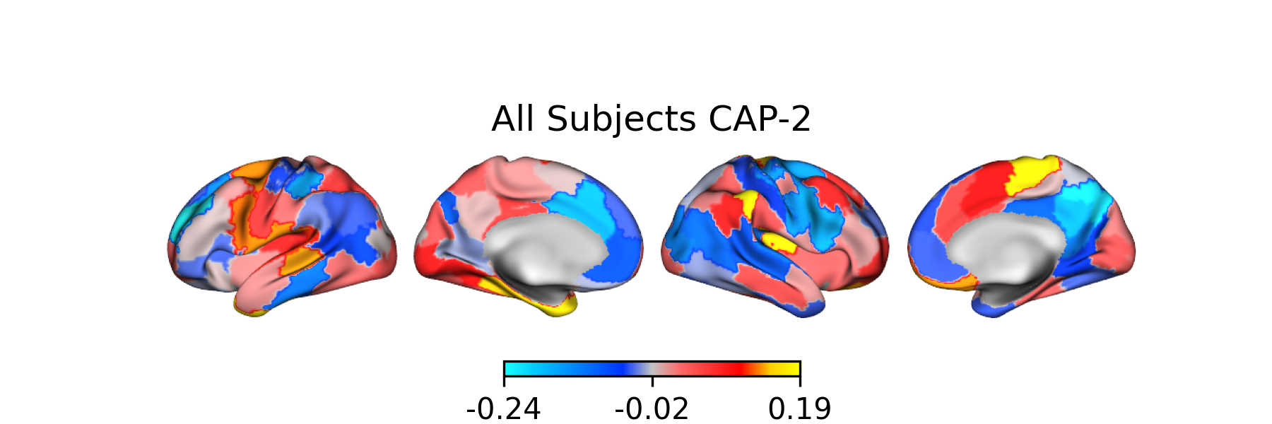
Creating Surface Plots#
from matplotlib.colors import LinearSegmentedColormap

# Create the colormap
colors = [
    "#1bfffe",
    "#00ccff",
    "#0099ff",
    "#0066ff",
    "#0033ff",
    "#c4c4c4",
    "#ff6666",
    "#ff3333",
    "#FF0000",
    "#ffcc00",
    "#FFFF00",
]

custom_cmap = LinearSegmentedColormap.from_list("custom_cold_hot", colors, N=256)

# Apply custom cmap to surface plots
cap_analysis.caps2surf(progress_bar=True, cmap=custom_cmap, size=(500, 100), layout="row")
Generating Surface Plots [GROUP: A]: 100%|█████████████████████████████████████████████████████████████████████████████████████████████████████████████████████████| 2/2 [00:07<00:00, 3.91s/it]
Generating Surface Plots [GROUP: B]: 100%|█████████████████████████████████████████████████████████████████████████████████████████████████████████████████████████| 2/2 [00:04<00:00, 2.12s/it]
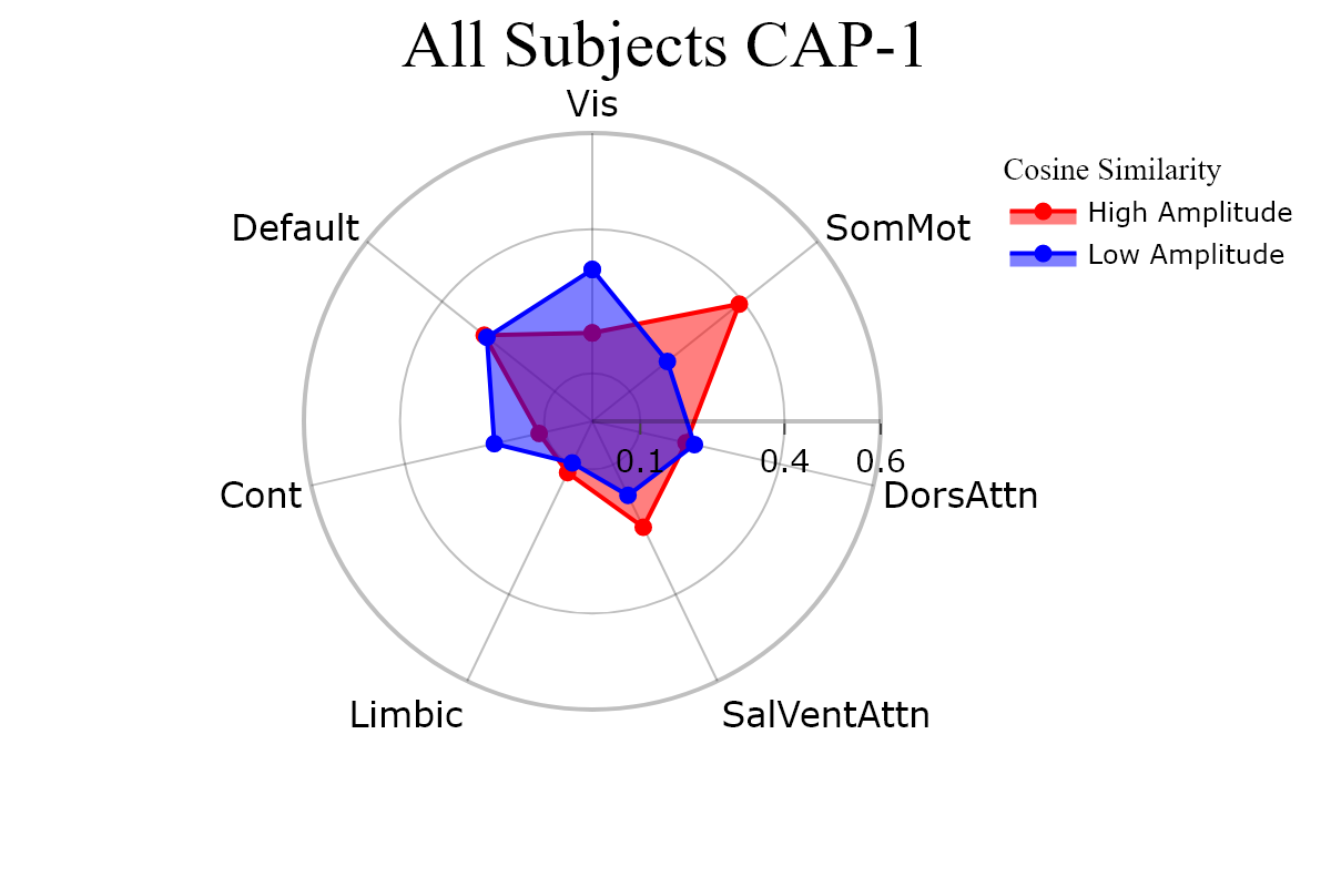
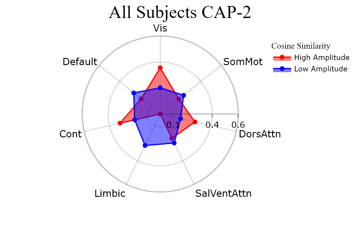
Plotting CAPs to Radar#
radialaxis = {
    "showline": True,
    "linewidth": 2,
    "linecolor": "rgba(0, 0, 0, 0.25)",
    "gridcolor": "rgba(0, 0, 0, 0.25)",
    "ticks": "outside",
    "tickfont": {"size": 14, "color": "black"},
    "range": [0, 0.6],
    "tickvals": [0.1, "", "", 0.4, "", "", 0.6],
}

legend = {
    "yanchor": "top",
    "y": 0.99,
    "x": 0.99,
    "title_font_family": "Times New Roman",
    "font": {"size": 12, "color": "black"},
}

colors = {"High Amplitude": "red", "Low Amplitude": "blue"}

kwargs = {
    "radialaxis": radialaxis,
    "fill": "toself",
    "legend": legend,
    "color_discrete_map": colors,
    "height": 400,
    "width": 600,
}

cap_analysis.caps2radar(**kwargs)