Tutorial 8: End-to-End CAPs Analysis Workflow#
![]()
![]()
This tutorial demonstrates how to use NeuroCAPs from timeseries extraction to CAPs visualization. Two subjects from a real, publicly available dataset are used so it may take a few minutes to download the files.
[ ]:
# Download packages
try:
    import neurocaps
except:
    !pip install neurocaps[windows,demo]

# Set headless display for google colab
import os, sys

if "google.colab" in sys.modules:
    os.environ["DISPLAY"] = ":0.0"
    !apt-get install -y xvfb
    !Xvfb :0 -screen 0 1024x768x24 &> /dev/null &
    !Xvfb :0 -screen 0 1024x768x24 &> /dev/null &
    !pip install jupyter_bokeh
    import IPython
    IPython.Application.instance().kernel.do_shutdown(True)
    !yes | plotly_get_chrome
[1]:
import os

demo_dir = "neurocaps_demo_workflow"
os.makedirs(demo_dir, exist_ok=True)
The code below fetches two subjects from an OpenNeuro dataset (from Chang et al. (2021)) preprocessed with fMRIPrep. Downloading data from OpenNeuro requires pip install openneuro-py ipywidgets or pip install neurocaps[demo].
[ ]:
# [Dataset] https://openneuro.org/datasets/ds003521/versions/2.2.0
from openneuro import download

# Include data from two subjects
include = [
    "dataset_description.json",
    "derivatives/fmriprep/dataset_description.json",
    "sub-sid000216/func/*events.tsv",
    "derivatives/fmriprep/sub-sid000216/func/*confounds_timeseries.tsv",
    "derivatives/fmriprep/sub-sid000216/func/*preproc_bold.nii.gz",
    "sub-sid000710/func/*events.tsv",
    "derivatives/fmriprep/sub-sid000710/func/*confounds_timeseries.tsv",
    "derivatives/fmriprep/sub-sid000710/func/*preproc_bold.nii.gz",
]

download(
    dataset="ds003521",
    include=include,
    target_dir=demo_dir,
    verify_hash=False,
    max_retries=10,
    max_concurrent_downloads=8,
)
👋 Hello! This is openneuro-py 2024.2.0. Great to see you! 🤗

   👉 Please report problems 🤯 and bugs 🪲 at
      https://github.com/hoechenberger/openneuro-py/issues

🌍 Preparing to download ds003521 …
📥 Retrieving up to 11 files (8 concurrent downloads).
✅ Finished downloading ds003521.

🧠 Please enjoy your brains.
The first level of the pipeline directory must also have a dataset_description.json file for querying purposes.
[2]:
import glob, os

# Ensure all files have the same run id if the "run-" entity is used.
for sub in ["sub-sid000216", "sub-sid000710"]:
    target_file = glob.glob(os.path.join(demo_dir, sub, "func", "*events.tsv"))[0]
    os.rename(target_file, target_file.replace("run-01", "run-1"))
[3]:
from neurocaps.extraction import TimeseriesExtractor
from neurocaps.utils import fetch_preset_parcel_approach

# List of fMRIPrep-derived confounds for nuisance regression
confound_names = [
    "cosine*",
    "trans_x",
    "trans_x_derivative1",
    "trans_y",
    "trans_y_derivative1",
    "trans_z",
    "trans_z_derivative1",
    "rot_x",
    "rot_x_derivative1",
    "rot_y",
    "rot_y_derivative1",
    "rot_z",
    "rot_z_derivative1",
    "a_comp_cor_00",
    "a_comp_cor_01",
    "a_comp_cor_02",
    "a_comp_cor_03",
    "a_comp_cor_04",
    "global_signal",
    "global_signal_derivative1",
]

# Initialize extractor with signal cleaning parameters
extractor = TimeseriesExtractor(
    space="MNI152NLin2009cAsym",
    parcel_approach=fetch_preset_parcel_approach("4S", n_nodes=456),
    standardize=True,
    confound_names=confound_names,
    fd_threshold={
        "threshold": 0.50,
        "outlier_percentage": 0.30,
    },
)

# Perform the timeseries extraction; only one session
# can be extracted at a time. Internally, lru_cache is used for
# ``BidsLayout``. May need to clear cache if the cell was ran
# before the directory download completed
try:
    TimeseriesExtractor._call_layout.cache_clear()
except:
    pass

# Extract BOLD data from preprocessed fMRIPrep data which should be located in
# the "derivatives" folder within the BIDS root directory.
# The extracted timeseries data is automatically stored
extractor.get_bold(
    bids_dir=demo_dir,
    task="movie",
    condition="Movie",
    condition_tr_shift=2,
    tr=2,
    n_cores=1,
    verbose=False,
).timeseries_to_pickle(demo_dir, "timeseries.pkl")
2025-07-30 17:37:02,619 neurocaps.extraction._internals.confounds [INFO] Confound regressors to be used if available: cosine*, trans_x, trans_x_derivative1, trans_y, trans_y_derivative1, trans_z, trans_z_derivative1, rot_x, rot_x_derivative1, rot_y, rot_y_derivative1, rot_z, rot_z_derivative1, a_comp_cor_00, a_comp_cor_01, a_comp_cor_02, a_comp_cor_03, a_comp_cor_04, global_signal, global_signal_derivative1.
2025-07-30 17:37:05,285 neurocaps.extraction.timeseries_extractor [INFO] BIDS Layout: ...orials\neurocaps_demo_workflow | Subjects: 2 | Sessions: 0 | Runs: 2
[3]:
<neurocaps.extraction.timeseries_extractor.TimeseriesExtractor at 0x194609c80d0>
[4]:
# Get dataframe of QC information to use for downstream statistical analyses
qc_df = extractor.report_qc()
qc_df
[4]:
| Subject_ID | Run | Mean_FD | Std_FD | Frames_Scrubbed | Frames_Interpolated | Mean_High_Motion_Length | Std_High_Motion_Length | N_Dummy_Scans | |
|---|---|---|---|---|---|---|---|---|---|
| 0 | sid000216 | run-1 | 0.082952 | 0.057038 | 2 | 0 | 1.00 | 0.000000 | NaN |
| 1 | sid000710 | run-1 | 0.083742 | 0.069571 | 5 | 0 | 1.25 | 0.433013 | NaN |
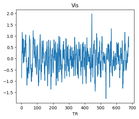
[5]:
# Visualize BOLD Data
from neurocaps.utils import PlotDefaults

plot_kwargs = PlotDefaults.visualize_bold()
plot_kwargs["figsize"] = (5, 4)

extractor.visualize_bold(subj_id="sid000216", run=1, region="Vis", **plot_kwargs)
[5]:
<neurocaps.extraction.timeseries_extractor.TimeseriesExtractor at 0x194609c80d0>
[6]:
from neurocaps.analysis import CAP
# Initialize CAP class
cap_analysis = CAP(parcel_approach=extractor.parcel_approach)
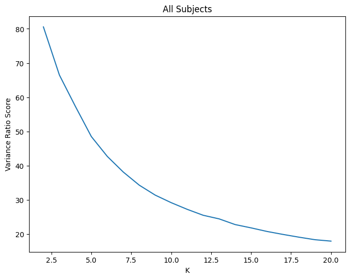
# Identify the optimal number of CAPs (clusters)
# using the variance_ratio method (higher score is better) to test 2-20
# The optimal number of CAPs is automatically stored
cap_analysis.get_caps(
subject_timeseries=extractor.subject_timeseries,
n_clusters=range(2, 21),
standardize=True,
cluster_selection_method="variance_ratio",
max_iter=500,
n_init=10,
random_state=0,
show_figs=True,
)
2025-07-30 17:37:32,313 neurocaps.analysis.cap._internals.cluster [INFO] No groups specified. Using default group 'All Subjects' containing all subject IDs from `subject_timeseries`. The `groups` dictionary will remain fixed unless the `CAP` class is re-initialized or `clear_groups()` is used.
2025-07-30 17:37:36,086 neurocaps.analysis.cap._internals.cluster [INFO] [GROUP: All Subjects | METHOD: variance_ratio] Optimal cluster size is 2.
[6]:
<neurocaps.analysis.cap.cap.CAP at 0x194624d4890>
Note that CAP-1 is the dominant brain state across subjects (highest frequency). However, a downstream statistical analysis should be conducted to determine the significance of this finding.
[7]:
# Calculate temporal fraction of each CAP for all subjects
output = cap_analysis.calculate_metrics(
    extractor.subject_timeseries, metrics=["temporal_fraction", "transition_probability"]
)
output["temporal_fraction"]
[7]:
| Subject_ID | Group | Run | CAP-1 | CAP-2 | |
|---|---|---|---|---|---|
| 0 | sid000216 | All Subjects | run-1 | 0.448378 | 0.551622 |
| 1 | sid000710 | All Subjects | run-1 | 0.422222 | 0.577778 |
[8]:
# Averaged transition probability matrix
from neurocaps.analysis import transition_matrix

df = transition_matrix(output["transition_probability"], return_df=True)
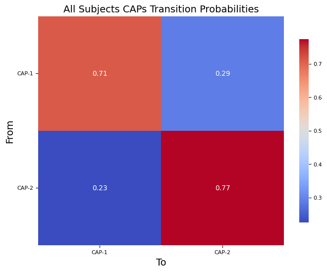
Note: Here CAP-1 is more likely to transition to itself than to CAP-2, likewise for CAP-2.
[9]:
df["All Subjects"]
[9]:
| CAP-1 | CAP-2 | |
|---|---|---|
| From/To | ||
| CAP-1 | 0.710204 | 0.289796 |
| CAP-2 | 0.226107 | 0.773893 |
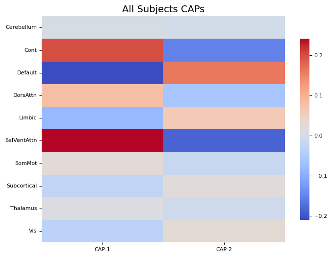
[10]:
cap_analysis.caps2plot(plot_options="heatmap")
[10]:
<neurocaps.analysis.cap.cap.CAP at 0x194624d4890>
Note: If the color_range kwarg is not used, each CAP will be scaled to its own maximum and minimum value. For directly comparable, zero-centered images, it is recommended to set a symmetric color_range based on the largest absolute value across all CAPs (e.g., if the largest absolute value is 0.96, use color_range=(-0.67, 0.67)).
[11]:
# Allow plotly to render correctly on static websites
import plotly.io as pio
pio.renderers.default = "svg"
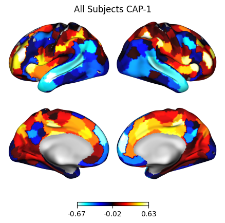
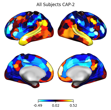
# Project CAPs onto surface plots and generate cosine similarity network alignment of CAPs
from neurocaps.utils import PlotDefaults
radialaxis = {
"showline": True,
"linewidth": 2,
"linecolor": "rgba(0, 0, 0, 0.25)",
"gridcolor": "rgba(0, 0, 0, 0.25)",
"ticks": "outside",
"tickfont": {"size": 14, "color": "black"},
"range": [0, 0.9],
"tickvals": [0.1, "", 0.3, "", 0.5, "", 0.7, "", 0.9],
}
color_discrete_map = {
"High Amplitude": "rgba(255, 165, 0, 0.75)",
"Low Amplitude": "black",
}
plot_kwargs = PlotDefaults.caps2radar()
plot_kwargs.update(dict(radialaxis=radialaxis, color_discrete_map=color_discrete_map))
cap_analysis.caps2surf().caps2radar(**plot_kwargs)


[11]:
<neurocaps.analysis.cap.cap.CAP at 0x194624d4890>
Radar plots show network alignment (measured by cosine similarity): “High Amplitude” = alignment to activations (> 0), “Low Amplitude” = alignment to deactivations (< 0).
Each CAP can be characterized using either maximum alignment (CAP-1: Vis+/SomMot-; CAP-2: SomMot+/Vis-) or predominant alignment (“High Amplitude” − “Low Amplitude”; CAP-1: SalVentAttn+/SomMot-; CAP-2: SomMot+/SalVentAttn-).
[13]:
import pandas as pd

for cap_name in cap_analysis.caps["All Subjects"]:
    df = pd.DataFrame(cap_analysis.cosine_similarity["All Subjects"][cap_name])
    # Note for "Low Amplitude" the absolute values of the
    # negative cosine similarities are stored
    df["Net"] = df["High Amplitude"] - df["Low Amplitude"]
    df["Regions"] = cap_analysis.cosine_similarity["All Subjects"]["Regions"]
    print(f"{cap_name}:", "\n", df, "\n")
CAP-1:
    High Amplitude  Low Amplitude       Net      Regions
0        0.049147       0.046088  0.003059   Cerebellum
1        0.415130       0.060391  0.354738         Cont
2        0.130936       0.619239 -0.488303      Default
3        0.235019       0.096929  0.138090     DorsAttn
4        0.034769       0.136324 -0.101555       Limbic
5        0.507167       0.098074  0.409093  SalVentAttn
6        0.143926       0.092124  0.051803       SomMot
7        0.024831       0.063271 -0.038440  Subcortical
8        0.030206       0.019487  0.010718     Thalamus
9        0.128041       0.192891 -0.064850          Vis

CAP-2:
    High Amplitude  Low Amplitude       Net      Regions
0        0.046088       0.049147 -0.003059   Cerebellum
1        0.060391       0.415130 -0.354738         Cont
2        0.619239       0.130936  0.488303      Default
3        0.096929       0.235019 -0.138090     DorsAttn
4        0.136324       0.034769  0.101555       Limbic
5        0.098074       0.507167 -0.409093  SalVentAttn
6        0.092124       0.143926 -0.051803       SomMot
7        0.063271       0.024831  0.038440  Subcortical
8        0.019487       0.030206 -0.010718     Thalamus
9        0.192891       0.128041  0.064850          Vis