Tutorial 2: Using neurocaps.analysis.CAP
Performing CAPs on All Subjects
from neurocaps.extraction import TimeseriesExtractor
from neurocaps.analysis import CAP
# Extracting timseries
parcel_approach = {"Schaefer": {"n_rois": 100, "yeo_networks": 7, "resolution_mm": 2}}
extractor = TimeseriesExtractor(parcel_approach=parcel_approach,
standardize="zscore_sample",
use_confounds=True,
detrend=True,
low_pass=0.15,
high_pass=0.01,
confound_names=confounds,
n_acompcor_separate=6)
extractor.get_bold(bids_dir=bids_dir,
task="emo",
condition="positive",
pipeline_name=pipeline_name,
n_cores=10)
# Saving timeseries
extractor.timeseries_to_pickle(output_dir="path/to/dir",
filename="task-positive_Schaefer.pkl")
# Initialize CAP class
cap_analysis = CAP()
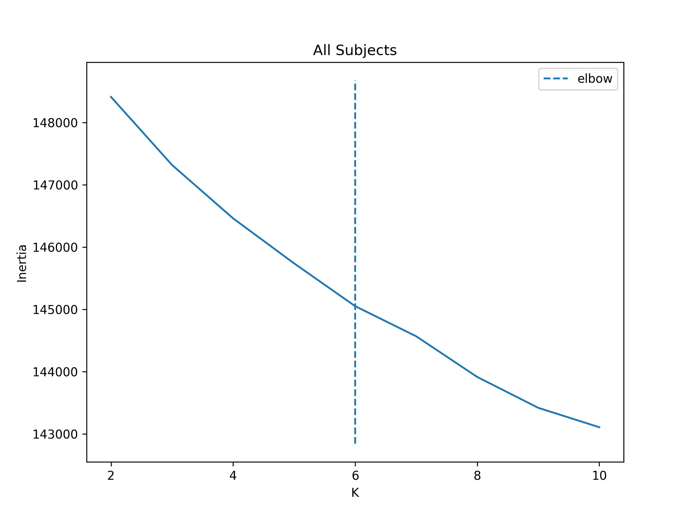
# Get CAPs
cap_analysis.get_caps(subject_timeseries=extractor.subject_timeseries,
n_clusters=range(2,11),
cluster_selection_method="elbow",
show_figs=True,
step=2)
2024-11-02 21:02:28,145 neurocaps.analysis.cap [INFO] [GROUP: All Subjects | METHOD: elbow] - Optimal cluster size is 6.
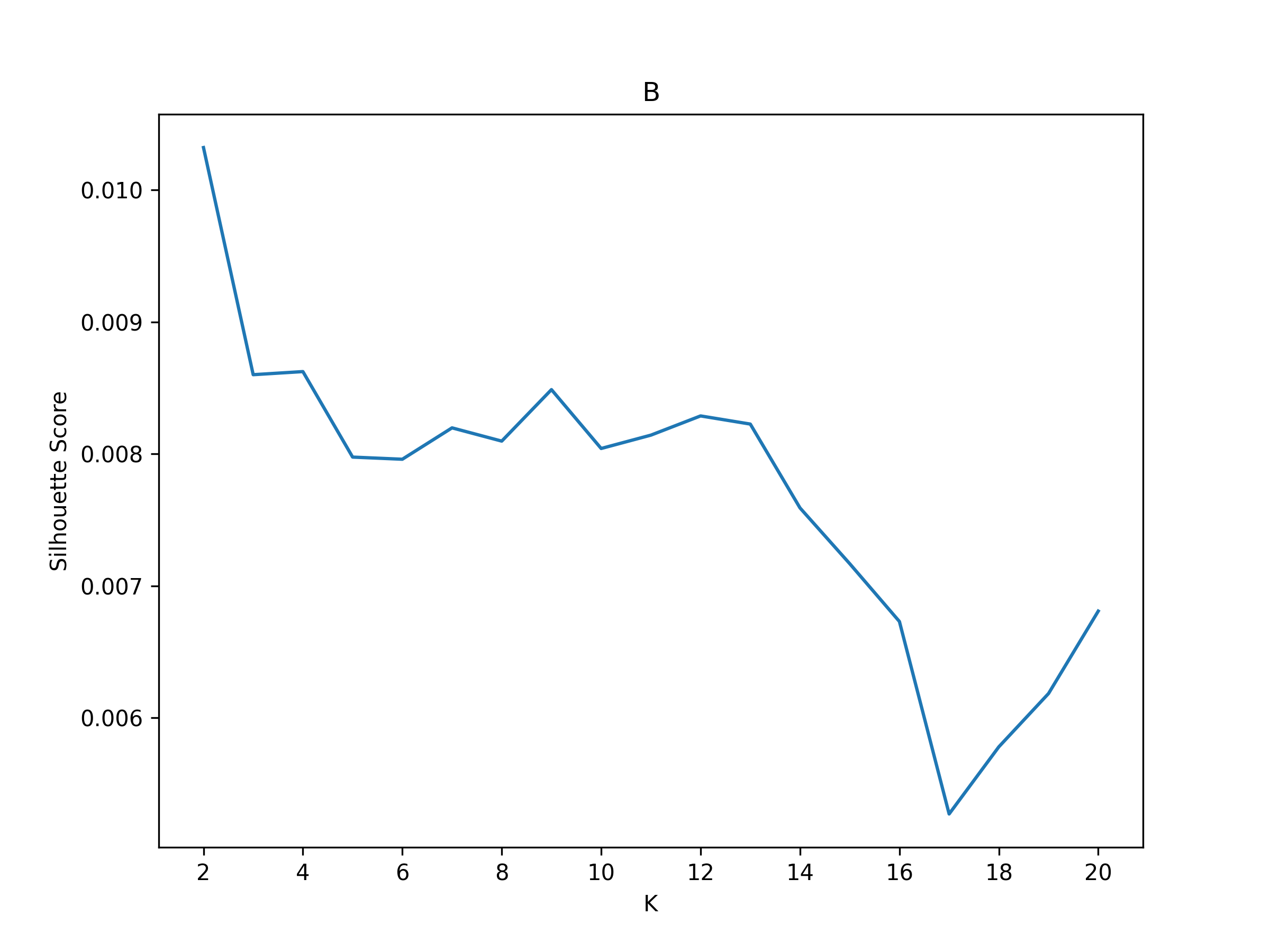
Performing CAPs on Groups
cap_analysis = CAP(groups={"A": ["1", "2", "3", "5"], "B": ["4", "6", "7", "8", "9", "10"]})

cap_analysis.get_caps(subject_timeseries="subject_timeseries.pkl",
                      n_clusters=range(2, 21),
                      cluster_selection_method="silhouette",
                      show_figs=True,
                      step=2)
2024-11-02 21:02:28,322 neurocaps.analysis.cap [INFO] [GROUP: A | METHOD: silhouette] - Optimal cluster size is 2.
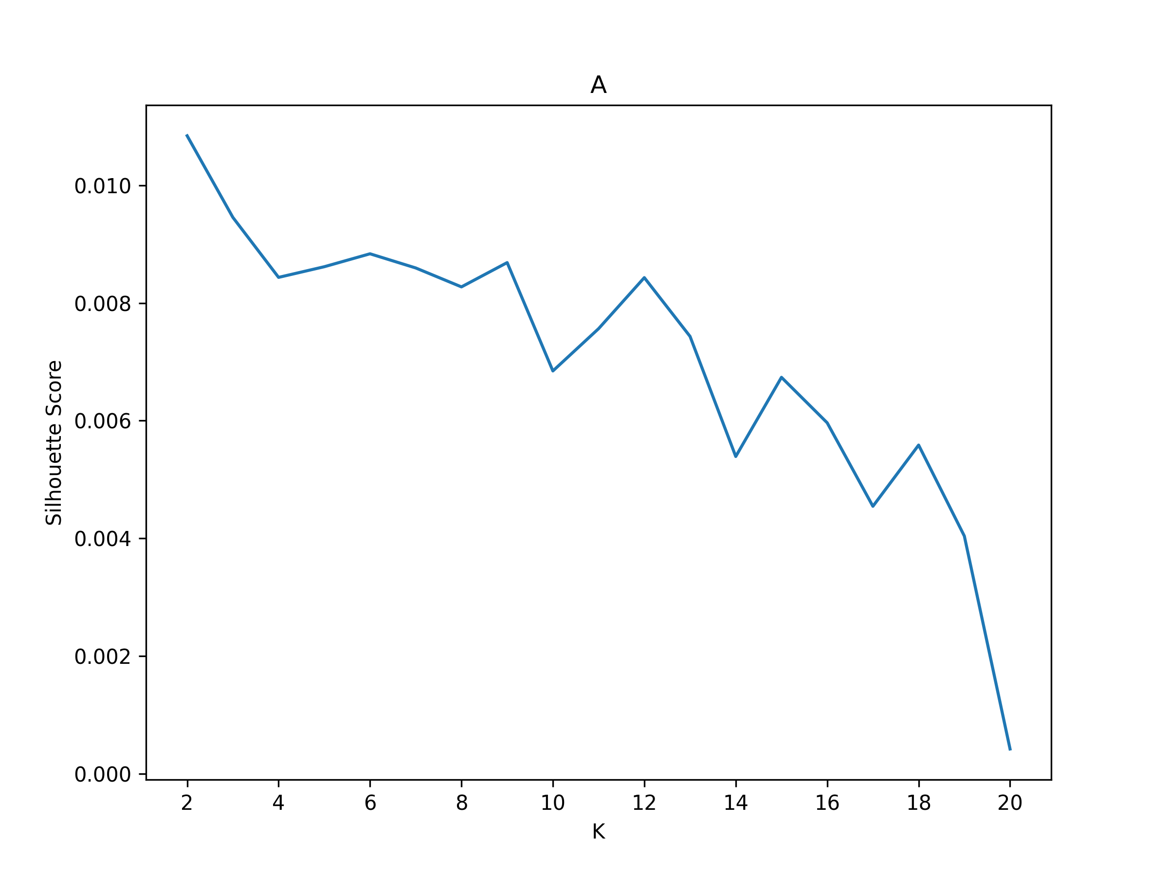
2024-11-02 21:02:28,541 neurocaps.analysis.cap [INFO] [GROUP: B | METHOD: silhouette] - Optimal cluster size is 2.
Calculate Metrics
df_dict = cap_analysis.calculate_metrics(subject_timeseries="subject_timeseries.pkl",
                                         return_df=True,
                                         metrics=["temporal_fraction", "counts", "transition_probability"],
                                         continuous_runs=True)

print(df_dict["temporal_fraction"])
Subject_ID |
Group |
Run |
CAP-1 |
CAP-2 |
|---|---|---|---|---|
1 |
A |
run-continuous |
0.5066666666666667 |
0.49333333333333335 |
2 |
A |
run-continuous |
0.5333333333333333 |
0.4666666666666667 |
3 |
A |
run-continuous |
0.6 |
0.4 |
5 |
A |
run-continuous |
0.54 |
0.46 |
4 |
B |
run-continuous |
0.41333333333333333 |
0.5866666666666667 |
6 |
B |
run-continuous |
0.47333333333333333 |
0.5266666666666666 |
7 |
B |
run-continuous |
0.44 |
0.56 |
8 |
B |
run-continuous |
0.5 |
0.5 |
9 |
B |
run-continuous |
0.4866666666666667 |
0.5133333333333333 |
10 |
B |
run-continuous |
0.46 |
0.54 |
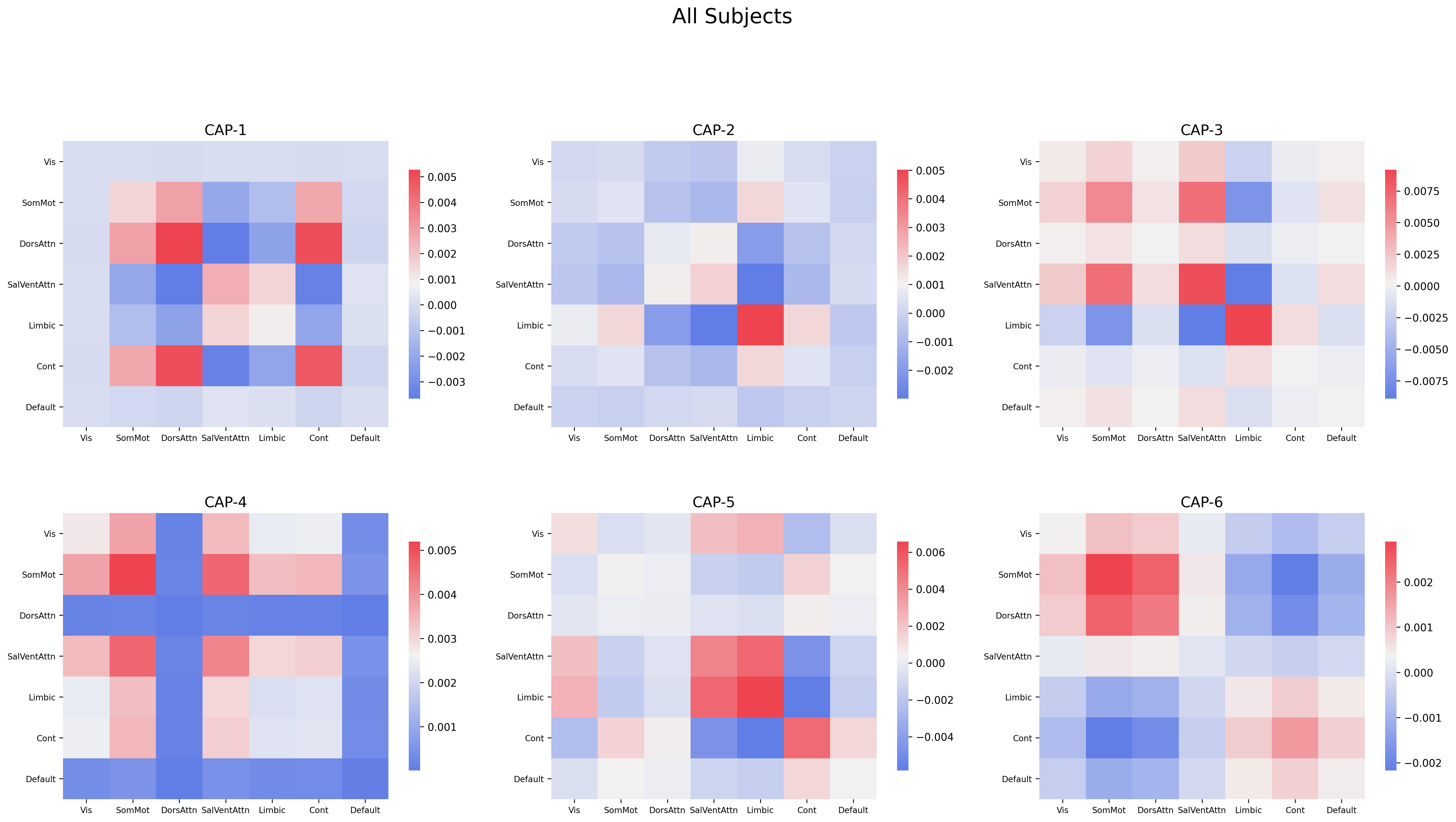
Plotting CAPs
import seaborn as sns

cap_analysis = CAP(parcel_approach=extractor.parcel_approach)

cap_analysis.get_caps(subject_timeseries=extractor.subject_timeseries,
                      n_clusters=6)

sns.diverging_palette(145, 300, s=60, as_cmap=True)

palette = sns.diverging_palette(260, 10, s=80, l=55, n=256, as_cmap=True)

kwargs = {"subplots": True, "fontsize": 14, "ncol": 3, "sharey": True,
          "tight_layout": False, "xlabel_rotation"L 0, "hspace": 0.3,
          "cmap": palette}

cap_analysis.caps2plot(visual_scope="regions",
                       plot_options="outer_product",
                       show_figs=True,
                       **kwargs)
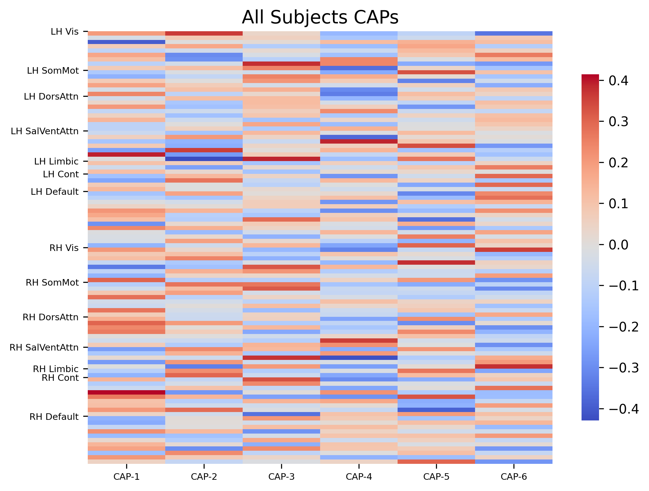
cap_analysis.caps2plot(visual_scope="nodes",
                       plot_options="heatmap",
                       xticklabels_size=7,
                       yticklabels_size=7,
                       show_figs=True)
Generate Pearson Correlation Matrix
cap_analysis.caps2corr(annot=True,
                       cmap="viridis",
                       show_figs=True)
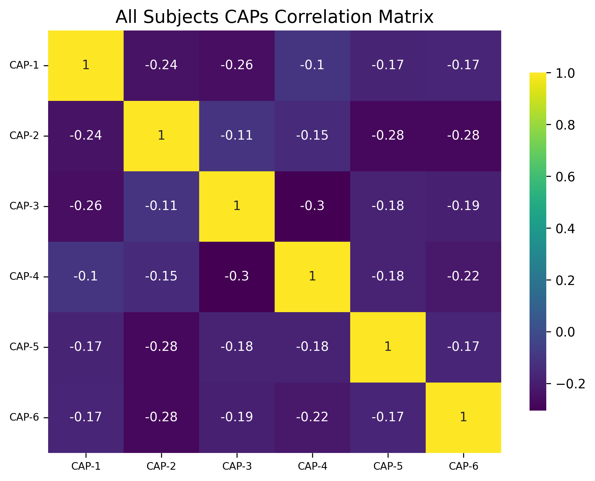
corr_dict = cap_analysis.caps2corr(return_df=True)
print(corr_dict["All Subjects"])
CAP-1 |
CAP-2 |
CAP-3 |
CAP-4 |
CAP-5 |
CAP-6 |
|
|---|---|---|---|---|---|---|
CAP-1 |
1 (0)*** |
-0.24 (0.016)* |
-0.26 (0.01)* |
-0.1 (0.3) |
-0.17 (0.087) |
-0.17 (0.09) |
CAP-2 |
-0.24 (0.016)* |
1 (0)*** |
-0.11 (0.28) |
-0.15 (0.14) |
-0.28 (0.0051)** |
-0.28 (0.0055)** |
CAP-3 |
-0.26 (0.01)* |
-0.11 (0.28) |
1 (0)*** |
-0.3 (0.0021)** |
-0.18 (0.075) |
-0.19 (0.058) |
CAP-4 |
-0.1 (0.3) |
-0.15 (0.14) |
-0.3 (0.0021)** |
1 (0)*** |
-0.18 (0.076) |
-0.22 (0.028)* |
CAP-5 |
-0.17 (0.087) |
-0.28 (0.0051)** |
-0.18 (0.075) |
-0.18 (0.076) |
1 (0)*** |
-0.17 (0.089) |
CAP-6 |
-0.17 (0.09) |
-0.28 (0.0055)** |
-0.19 (0.058) |
-0.22 (0.028)* |
-0.17 (0.089) |
1 (0)*** |
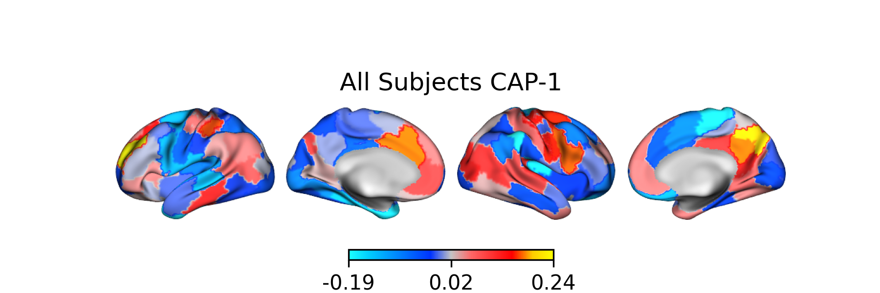
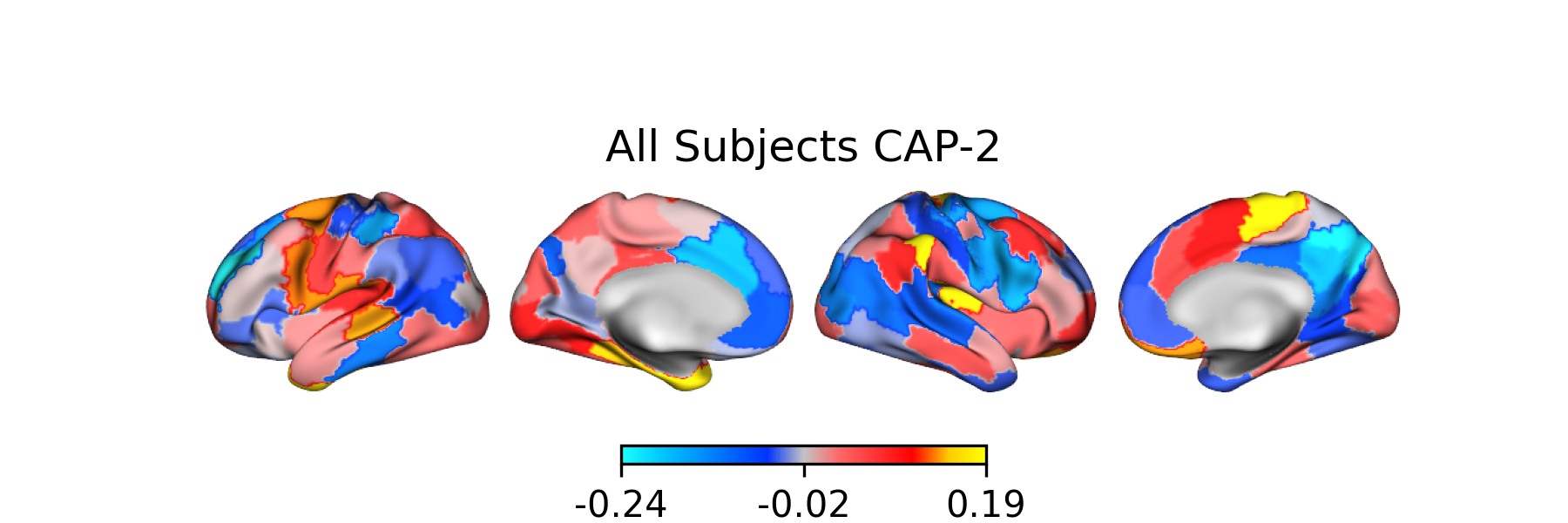
Creating Surface Plots
from matplotlib.colors import LinearSegmentedColormap

# Create the colormap
colors = ["#1bfffe", "#00ccff", "#0099ff", "#0066ff", "#0033ff", "#c4c4c4", "#ff6666",
          "#ff3333", "#FF0000","#ffcc00","#FFFF00"]

custom_cmap = LinearSegmentedColormap.from_list("custom_cold_hot", colors, N=256)

# Apply custom cmap to surface plots
cap_analysis.caps2surf(cmap=custom_cmap,
                       size=(500, 100),
                       layout="row")
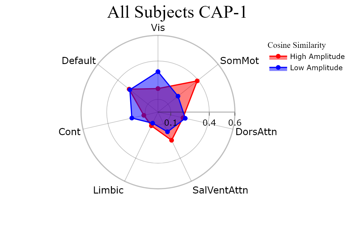
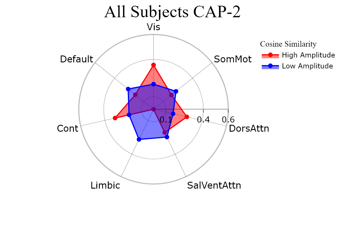
Plotting CAPs to Radar
radialaxis={"showline": True,
            "linewidth": 2,
            "linecolor": "rgba(0, 0, 0, 0.25)",
            "gridcolor": "rgba(0, 0, 0, 0.25)",
            "ticks": "outside" ,
            "tickfont": {"size": 14, "color": "black"},
            "range": [0, 0.6],
            "tickvals": [0.1, "", "", 0.4, "", "", 0.6]}

legend = {"yanchor": "top",
          "y": 0.99,
          "x": 0.99,
          "title_font_family": "Times New Roman",
          "font": {"size": 12, "color": "black"}}

colors =  {"High Amplitude": "red", "Low Amplitude": "blue"}


kwargs = {"radialaxis": radial, "fill": "toself", "legend": legend,
          "color_discrete_map": colors, "height": 400, "width": 600}

cap_analysis.caps2radar(**kwargs)