Tutorial 2: Using `neurocaps.analysis.CAP`

The CAP class is designed to perform CAP analyses (on all subjects or group of subjects). It offers the flexibility to analyze data from all subjects or focus on specific groups, compute CAP-specific metrics, and generate visualizations to aid in the interpretation of results.

Performing CAPs on All Subjects

import numpy as np
from neurocaps.analysis import CAP

# Extracting timseries
parcel_approach = {"Schaefer": {"n_rois": 100, "yeo_networks": 7, "resolution_mm": 2}}

# Simulate data for example
subject_timeseries = {str(x): {f"run-{y}": np.random.rand(100, 100) for y in range(1, 4)} for x in range(1, 11)}

# Initialize CAP class
cap_analysis = CAP(parcel_approach=parcel_approach)

# Get CAPs
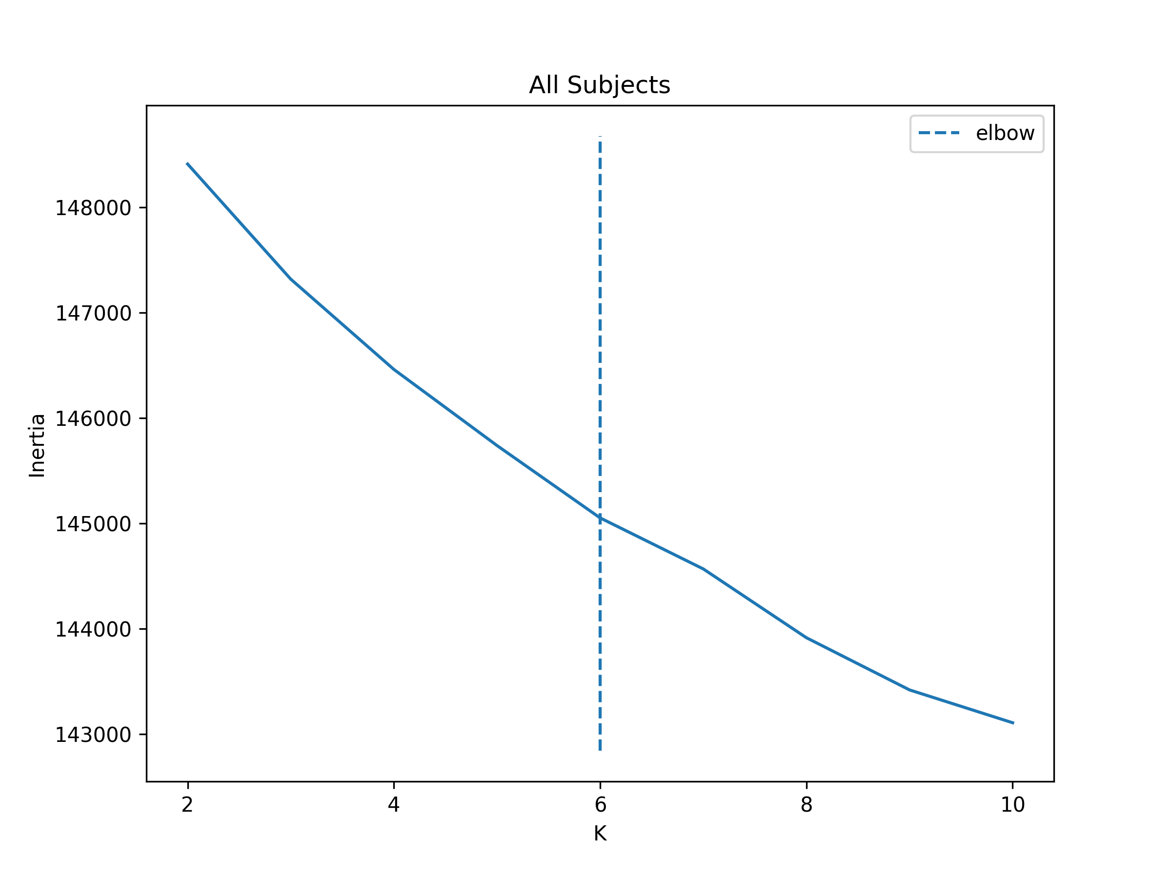
cap_analysis.get_caps(
    subject_timeseries=subject_timeseries,
    n_clusters=range(2, 11),
    cluster_selection_method="elbow",
    show_figs=True,
    step=2,
    progress_bar=True,  # Available in versions >= 0.21.5
)

Clustering [GROUP: All Subjects]: 100%|████████████████████████████████████████████████████████████████████████████████████████████████████████████████████████████| 9/9 [00:00<00:00, 20.38it/s]
2025-01-31 13:28:43,571 neurocaps.analysis.cap [INFO] [GROUP: All Subjects | METHOD: elbow] Optimal cluster size is 6.

../_images/All_Subjects_elbow.png

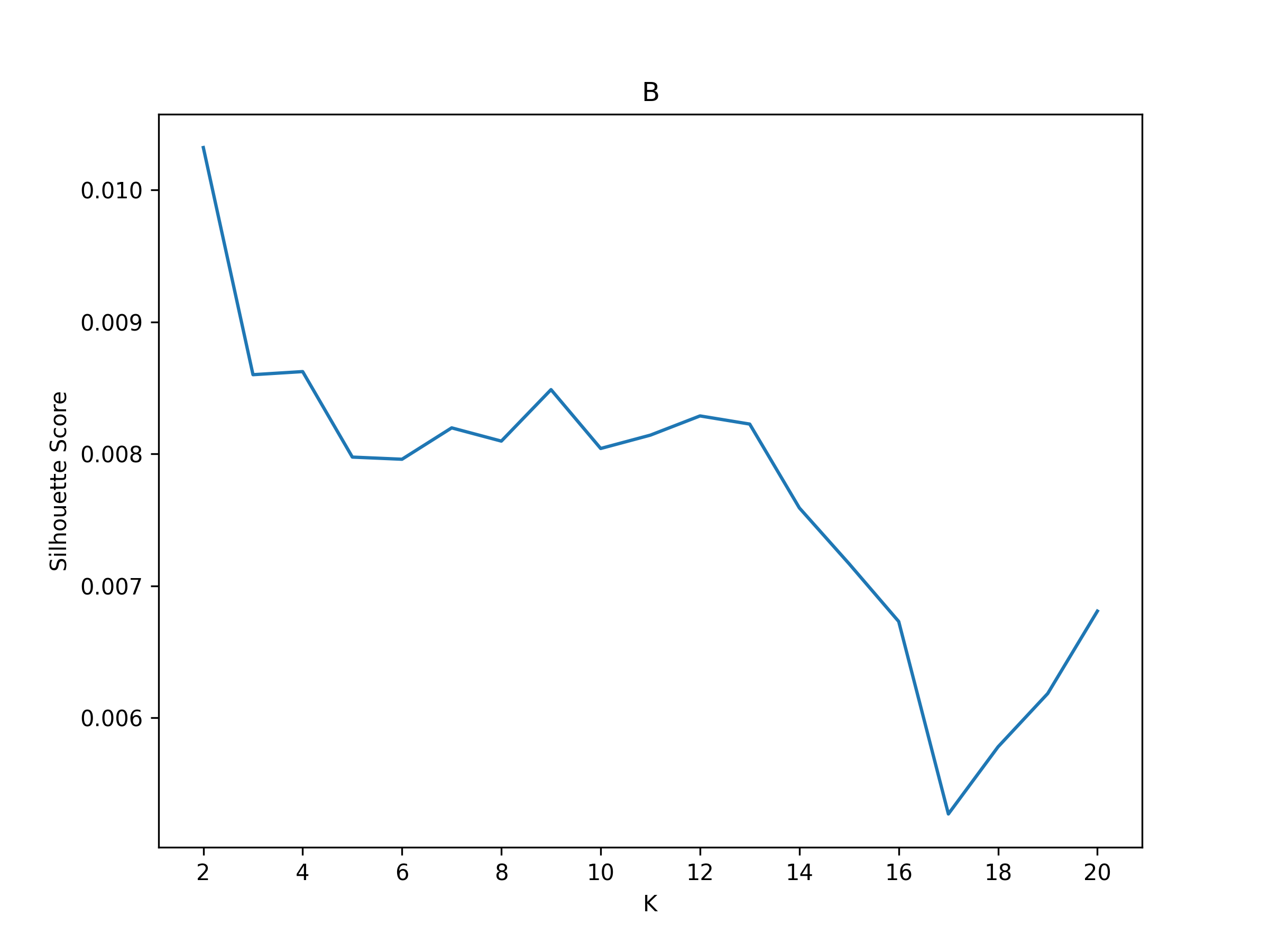
Performing CAPs on Groups

cap_analysis = CAP(groups={"A": ["1", "2", "3", "5"], "B": ["4", "6", "7", "8", "9", "10"]})

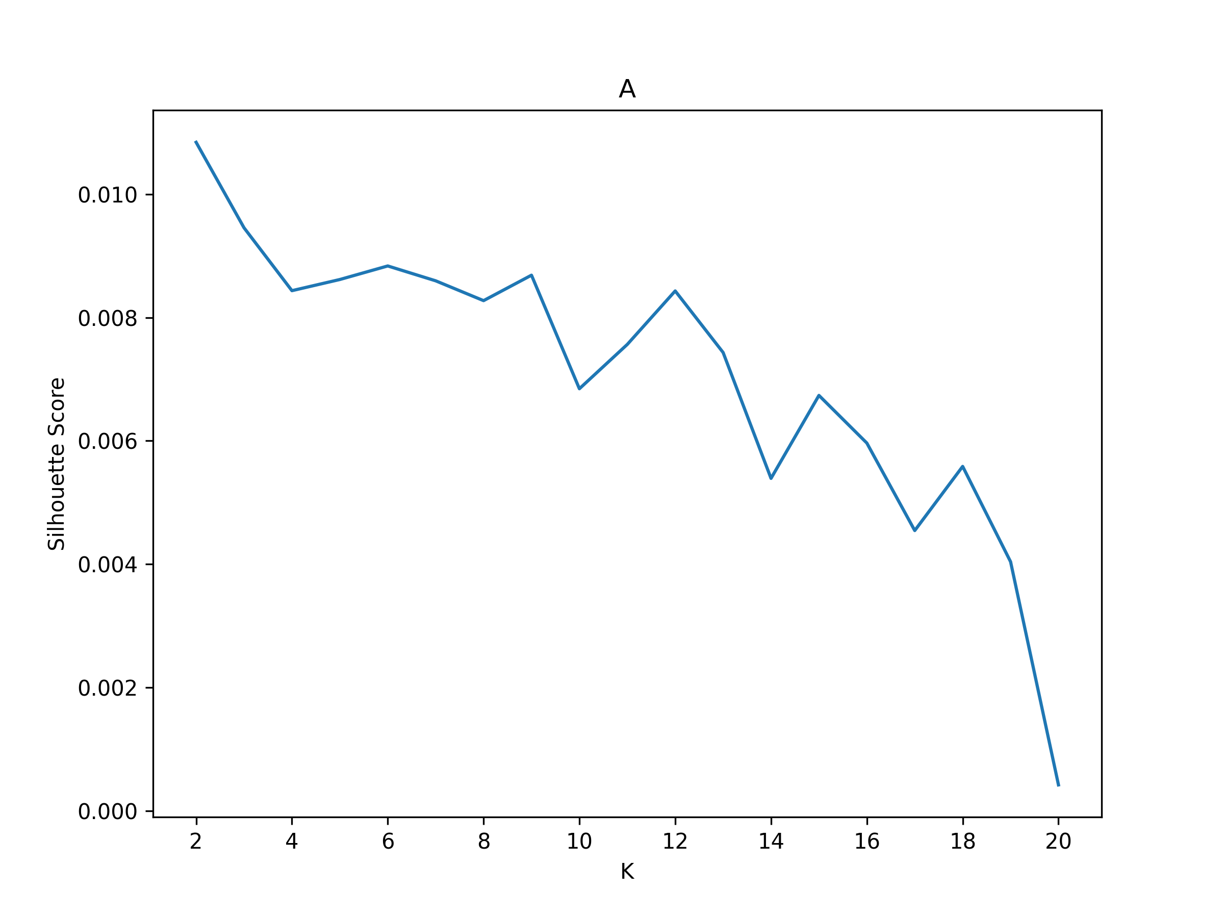
cap_analysis.get_caps(
    subject_timeseries=subject_timeseries,
    n_clusters=range(2, 21),
    cluster_selection_method="silhouette",
    show_figs=True,
    step=2,
    progress_bar=True,
)

Clustering [GROUP: A]: 100%|█████████████████████████████████████████████████████████████████████████████████████████████████████████████████████████████████████| 19/19 [00:01<00:00, 18.71it/s]
2025-01-31 13:29:54,234 neurocaps.analysis.cap [INFO] [GROUP: A | METHOD: silhouette] Optimal cluster size is 2.

../_images/A_silhouette.png

Clustering [GROUP: B]: 100%|█████████████████████████████████████████████████████████████████████████████████████████████████████████████████████████████████████| 19/19 [00:01<00:00, 12.48it/s]
2025-01-31 13:29:57,757 neurocaps.analysis.cap [INFO] [GROUP: B | METHOD: silhouette] Optimal cluster size is 2.

../_images/B_silhouette.png

Calculate Metrics

df_dict = cap_analysis.calculate_metrics(
    subject_timeseries=subject_timeseries,
    return_df=True,
    metrics=["temporal_fraction", "counts", "transition_probability"],
    continuous_runs=True,
    progress_bar=True,
)

print(df_dict["temporal_fraction"])

Computing Metrics for Subjects: 100%|███████████████████████████████████████████████████████████████████████████████████████████████████████████████████████████| 10/10 [00:00<00:00, 159.78it/s]

Subject_ID	Group	Run	CAP-1	CAP-2
1	A	run-continuous	0.5066666666666667	0.49333333333333335
2	A	run-continuous	0.5333333333333333	0.4666666666666667
3	A	run-continuous	0.6	0.4
5	A	run-continuous	0.54	0.46
4	B	run-continuous	0.41333333333333333	0.5866666666666667
6	B	run-continuous	0.47333333333333333	0.5266666666666666
7	B	run-continuous	0.44	0.56
8	B	run-continuous	0.5	0.5
9	B	run-continuous	0.4866666666666667	0.5133333333333333
10	B	run-continuous	0.46	0.54

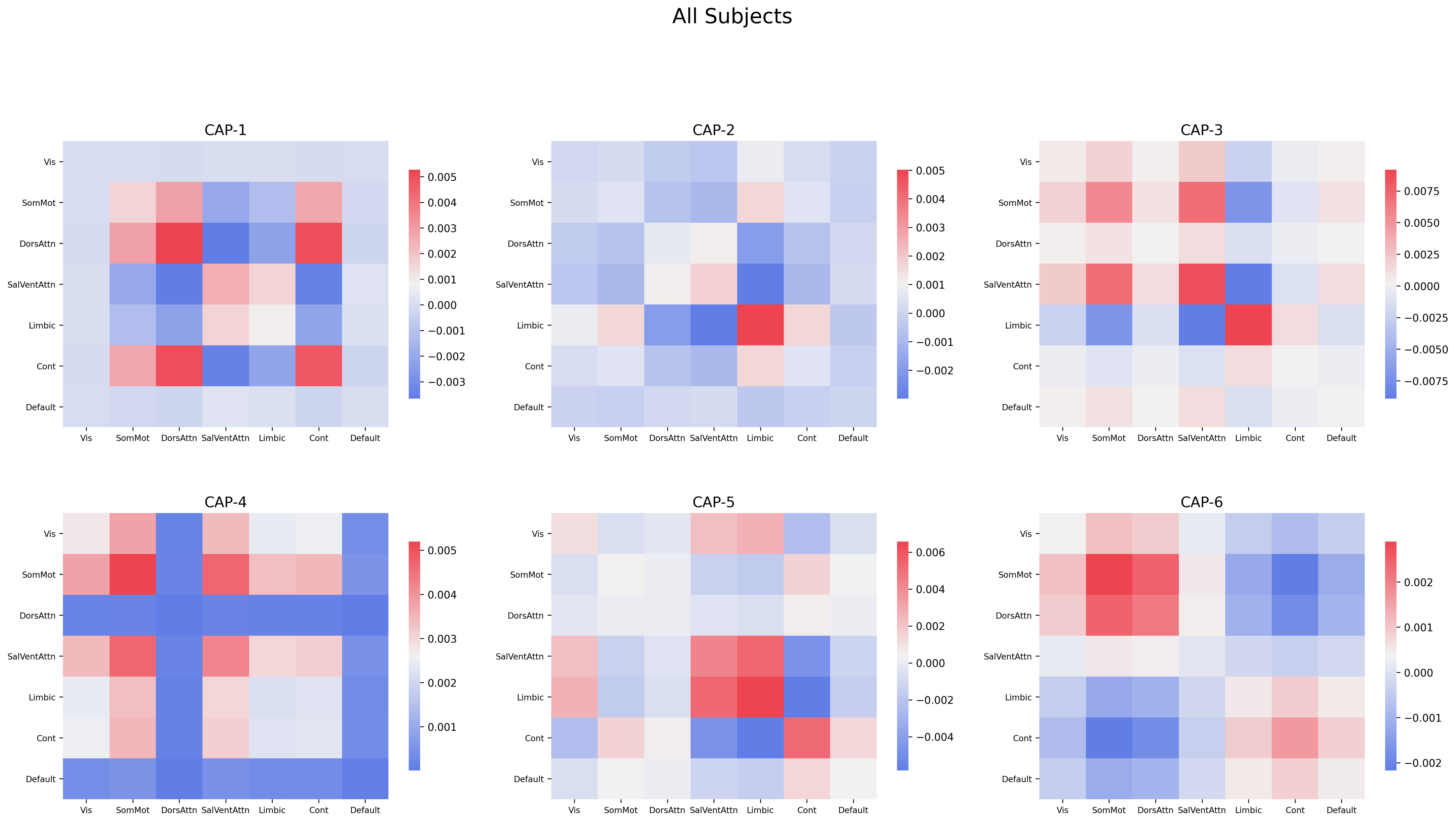
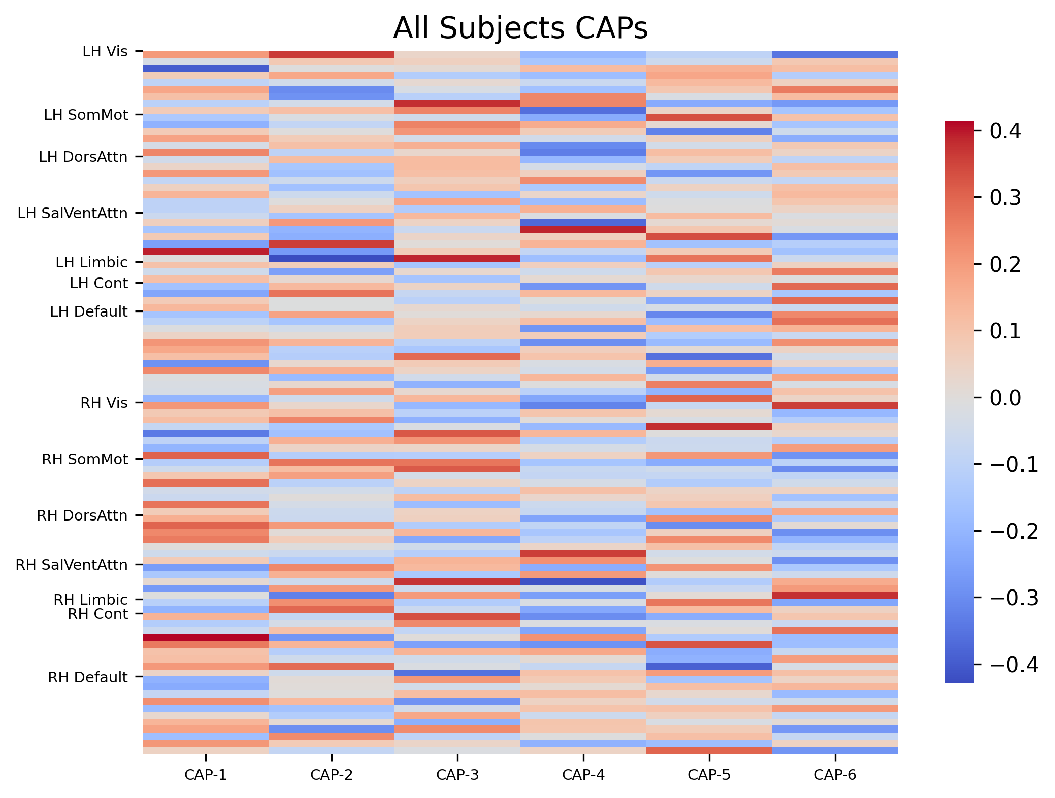
Plotting CAPs

import seaborn as sns

cap_analysis = CAP(parcel_approach=extractor.parcel_approach)

cap_analysis.get_caps(subject_timeseries=subject_timeseries, n_clusters=6)

sns.diverging_palette(145, 300, s=60, as_cmap=True)

palette = sns.diverging_palette(260, 10, s=80, l=55, n=256, as_cmap=True)

kwargs = {
    "subplots": True,
    "fontsize": 14,
    "ncol": 3,
    "sharey": True,
    "tight_layout": False,
    "xlabel_rotation": 0,
    "hspace": 0.3,
    "cmap": palette,
}

cap_analysis.caps2plot(visual_scope="regions", plot_options="outer_product", show_figs=True, **kwargs)

../_images/All_Subjects_CAPs_outer_product_heatmap-regions.png

cap_analysis.caps2plot(
    visual_scope="nodes", plot_options="heatmap", xticklabels_size=7, yticklabels_size=7, show_figs=True
)

../_images/All_Subjects_CAPs_heatmap-nodes.png

Generate Pearson Correlation Matrix

cap_analysis.caps2corr(annot=True, cmap="viridis", show_figs=True)

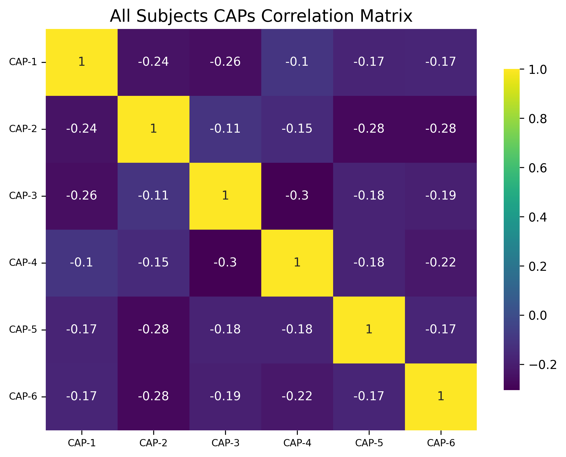
../_images/All_Subjects_CAPs_correlation_matrix.png

corr_dict = cap_analysis.caps2corr(return_df=True)
print(corr_dict["All Subjects"])

	CAP-1	CAP-2	CAP-3	CAP-4	CAP-5	CAP-6
CAP-1	1 (0)***	-0.24 (0.016)*	-0.26 (0.01)*	-0.1 (0.3)	-0.17 (0.087)	-0.17 (0.09)
CAP-2	-0.24 (0.016)*	1 (0)***	-0.11 (0.28)	-0.15 (0.14)	-0.28 (0.0051)**	-0.28 (0.0055)**
CAP-3	-0.26 (0.01)*	-0.11 (0.28)	1 (0)***	-0.3 (0.0021)**	-0.18 (0.075)	-0.19 (0.058)
CAP-4	-0.1 (0.3)	-0.15 (0.14)	-0.3 (0.0021)**	1 (0)***	-0.18 (0.076)	-0.22 (0.028)*
CAP-5	-0.17 (0.087)	-0.28 (0.0051)**	-0.18 (0.075)	-0.18 (0.076)	1 (0)***	-0.17 (0.089)
CAP-6	-0.17 (0.09)	-0.28 (0.0055)**	-0.19 (0.058)	-0.22 (0.028)*	-0.17 (0.089)	1 (0)***

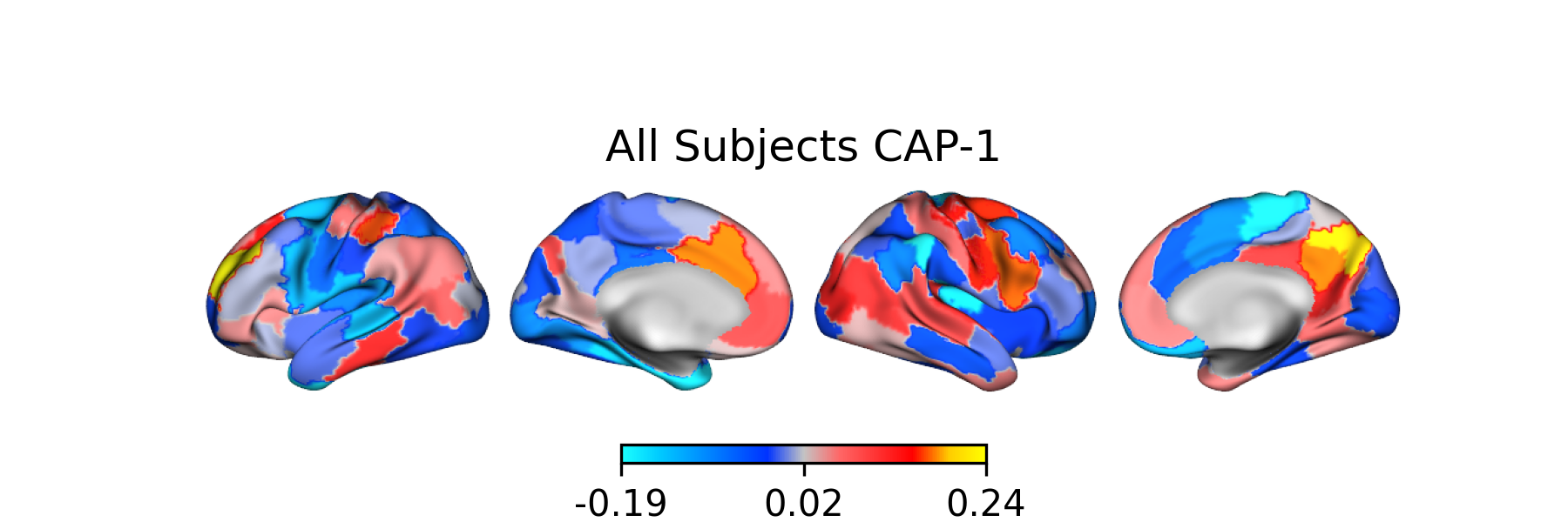
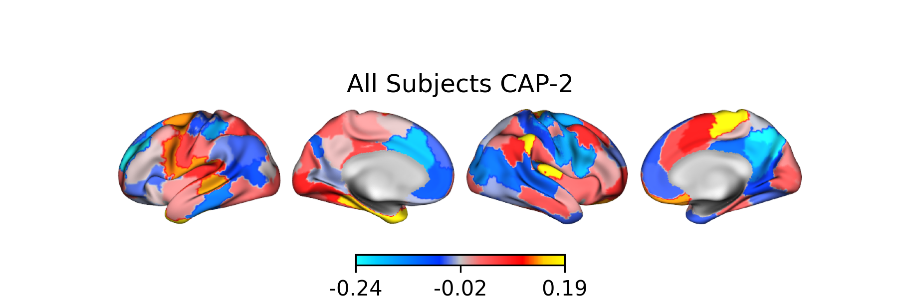
Creating Surface Plots

from matplotlib.colors import LinearSegmentedColormap

# Create the colormap
colors = [
    "#1bfffe",
    "#00ccff",
    "#0099ff",
    "#0066ff",
    "#0033ff",
    "#c4c4c4",
    "#ff6666",
    "#ff3333",
    "#FF0000",
    "#ffcc00",
    "#FFFF00",
]

custom_cmap = LinearSegmentedColormap.from_list("custom_cold_hot", colors, N=256)

# Apply custom cmap to surface plots
cap_analysis.caps2surf(progress_bar=True, cmap=custom_cmap, size=(500, 100), layout="row")

Generating Surface Plots [GROUP: A]: 100%|█████████████████████████████████████████████████████████████████████████████████████████████████████████████████████████| 2/2 [00:07<00:00,  3.91s/it]

../_images/All_Subjects_CAP-1_surface_plot.png

Generating Surface Plots [GROUP: B]: 100%|█████████████████████████████████████████████████████████████████████████████████████████████████████████████████████████| 2/2 [00:04<00:00,  2.12s/it]

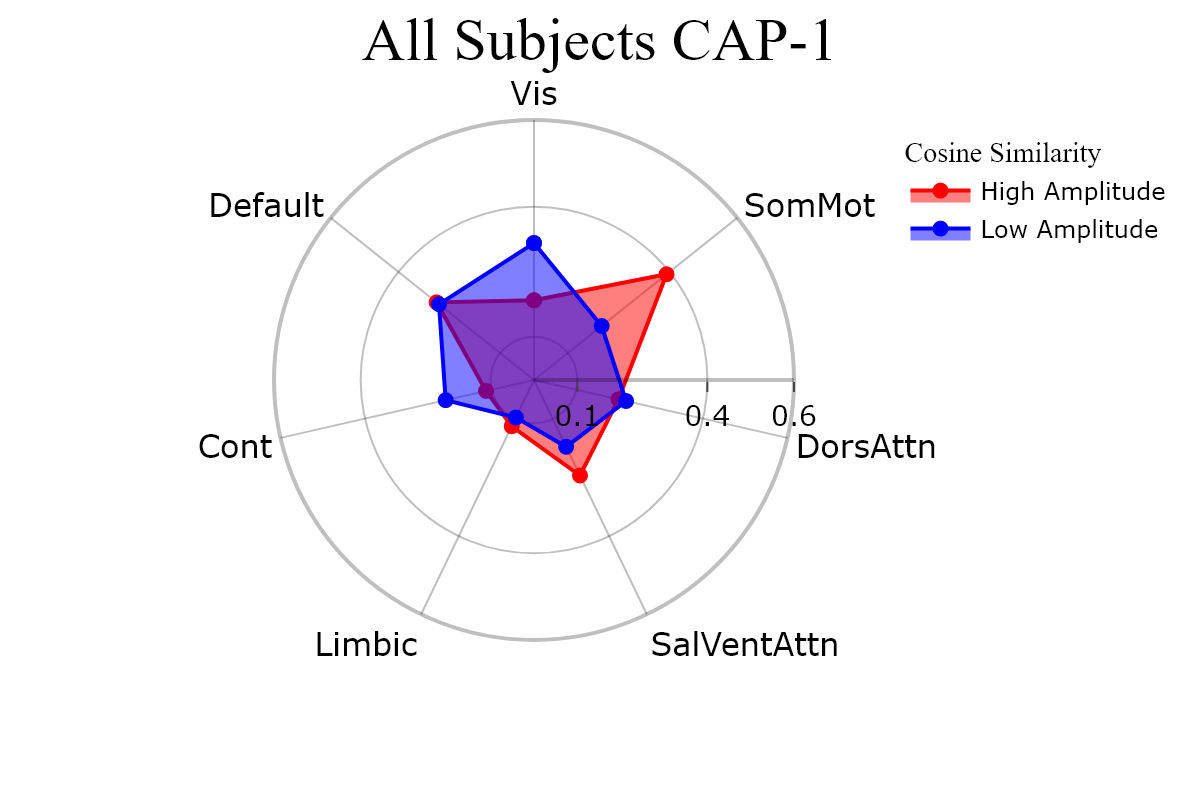
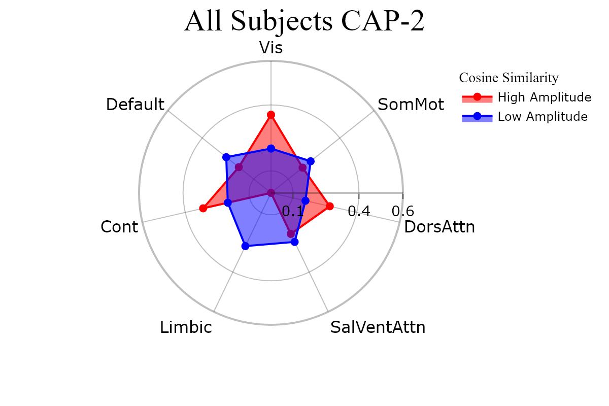
../_images/All_Subjects_CAP-2_surface_plot.png

Plotting CAPs to Radar

radialaxis = {
    "showline": True,
    "linewidth": 2,
    "linecolor": "rgba(0, 0, 0, 0.25)",
    "gridcolor": "rgba(0, 0, 0, 0.25)",
    "ticks": "outside",
    "tickfont": {"size": 14, "color": "black"},
    "range": [0, 0.6],
    "tickvals": [0.1, "", "", 0.4, "", "", 0.6],
}

legend = {
    "yanchor": "top",
    "y": 0.99,
    "x": 0.99,
    "title_font_family": "Times New Roman",
    "font": {"size": 12, "color": "black"},
}

colors = {"High Amplitude": "red", "Low Amplitude": "blue"}

kwargs = {
    "radialaxis": radial,
    "fill": "toself",
    "legend": legend,
    "color_discrete_map": colors,
    "height": 400,
    "width": 600,
}

cap_analysis.caps2radar(**kwargs)

../_images/All_Subjects_CAP-1_radar.png

../_images/All_Subjects_CAP-2_radar.png