Tutorial 8: Workflow Example#
![]()
This tutorial demonstrates an example workflow from timeseries extraction to CAPs visualization. Two subjects from a real, publicly available dataset are used so it may take a few minutes to download the files.
import os

demo_dir = "neurocaps_demo"
os.makedirs(demo_dir, exist_ok=True)
The code below fetches two subjects from an OpenNeuro dataset
preprocessed with fMRIPrep. Downloading data from OpenNeuro requires
pip install openneuro-py ipywidgets or pip install neurocaps[demo].
# [Dataset] doi: doi:10.18112/openneuro.ds005381.v1.0.0
from openneuro import download

# Include the run-1 and run-2 data from two subjects
include = [
    "dataset_description.json",
    "sub-0004/ses-2/func/*run-[12]*events*",
    "derivatives/fmriprep/sub-0004/fmriprep/sub-0004/ses-2/func/*run-[12]*confounds_timeseries*",
    "derivatives/fmriprep/sub-0004/fmriprep/sub-0004/ses-2/func/*run-[12]_space-MNI152NLin*preproc_bold*",
    "sub-0006/ses-2/func/*run-[12]*events*",
    "derivatives/fmriprep/sub-0006/fmriprep/sub-0006/ses-2/func/*run-[12]*confounds_timeseries*",
    "derivatives/fmriprep/sub-0006/fmriprep/sub-0006/ses-2/func/*run-[12]_space-MNI152NLin*preproc_bold*",
]

download(
    dataset="ds005381",
    include=include,
    target_dir=demo_dir,
    verify_hash=False,
)
The first level of the pipeline directory must also have a “dataset_description.json” file for querying purposes.
import json

desc = {
    "Name": "fMRIPrep - fMRI PREProcessing workflow",
    "BIDSVersion": "1.0.0",
    "DatasetType": "derivative",
    "GeneratedBy": [
        {"Name": "fMRIPrep", "Version": "20.2.0", "CodeURL": "https://github.com/nipreps/fmriprep"}
    ],
}

with open(
    "neurocaps_demo/derivatives/fmriprep/dataset_description.json", "w", encoding="utf-8"
) as f:
    json.dump(desc, f)
from neurocaps.extraction import TimeseriesExtractor
from neurocaps.utils import fetch_preset_parcel_approach

# List of fMRIPrep-derived confounds for nuisance regression
confound_names = [
    "cosine*",
    "trans_x",
    "trans_x_derivative1",
    "trans_y",
    "trans_y_derivative1",
    "trans_z",
    "trans_z_derivative1",
    "rot_x",
    "rot_x_derivative1",
    "rot_y",
    "rot_y_derivative1",
    "rot_z",
    "rot_z_derivative1",
    "a_comp_cor_00",
    "a_comp_cor_01",
    "a_comp_cor_02",
    "a_comp_cor_03",
    "a_comp_cor_04",
    "global_signal",
    "global_signal_derivative1",
]

# Initialize extractor with signal cleaning parameters
extractor = TimeseriesExtractor(
    space="MNI152NLin6Asym",
    parcel_approach=fetch_preset_parcel_approach("4S", n_nodes=456),
    standardize=True,
    confound_names=confound_names,
    fd_threshold={
        "threshold": 0.50,
        "outlier_percentage": 0.30,
    },
)

# Extract BOLD data from preprocessed fMRIPrep data
# which should be located in the "derivatives" folder
# within the BIDS root directory
# The extracted timeseries data is automatically stored
# Session 2 is the only session available, so `session`
# does not need to be specified
extractor.get_bold(
    bids_dir=demo_dir,
    task="DET",
    condition="late",
    condition_tr_shift=4,
    tr=2,
    verbose=False,
).timeseries_to_pickle(demo_dir, "timeseries.pkl")
2025-07-08 08:21:36,497 neurocaps.extraction._internals.confounds [INFO] Confound regressors to be used if available: cosine*, trans_x, trans_x_derivative1, trans_y, trans_y_derivative1, trans_z, trans_z_derivative1, rot_x, rot_x_derivative1, rot_y, rot_y_derivative1, rot_z, rot_z_derivative1, a_comp_cor_00, a_comp_cor_01, a_comp_cor_02, a_comp_cor_03, a_comp_cor_04, global_signal, global_signal_derivative1.
2025-07-08 08:21:38,133 neurocaps.extraction.timeseries_extractor [INFO] BIDS Layout: ...mples\notebooks\neurocaps_demo | Subjects: 2 | Sessions: 2 | Runs: 4
# Retrieve the dataframe containing QC information for each subject
# to use for downstream statistical analyses
qc_df = extractor.report_qc()
print(qc_df)
Subject_ID |
Run |
Mean_FD |
Std_FD |
Frames_Scrubbed |
Frames_Interpolated |
Mean_High_Motion_Length |
Std_High_Motion_Length |
N_Dummy_Scans |
|---|---|---|---|---|---|---|---|---|
0004 |
run-1 |
0.13200761871428568 |
0.14254231139501328 |
1 |
0 |
1.0 |
0.0 |
|
0004 |
run-2 |
0.10379914769230766 |
0.05579349376314367 |
0 |
0 |
0.0 |
0.0 |
|
0006 |
run-1 |
0.15367701594594593 |
0.0991528154121092 |
0 |
0 |
0.0 |
0.0 |
|
0006 |
run-2 |
0.1524833347354838 |
0.07865715802131876 |
0 |
0 |
0.0 |
0.0 |
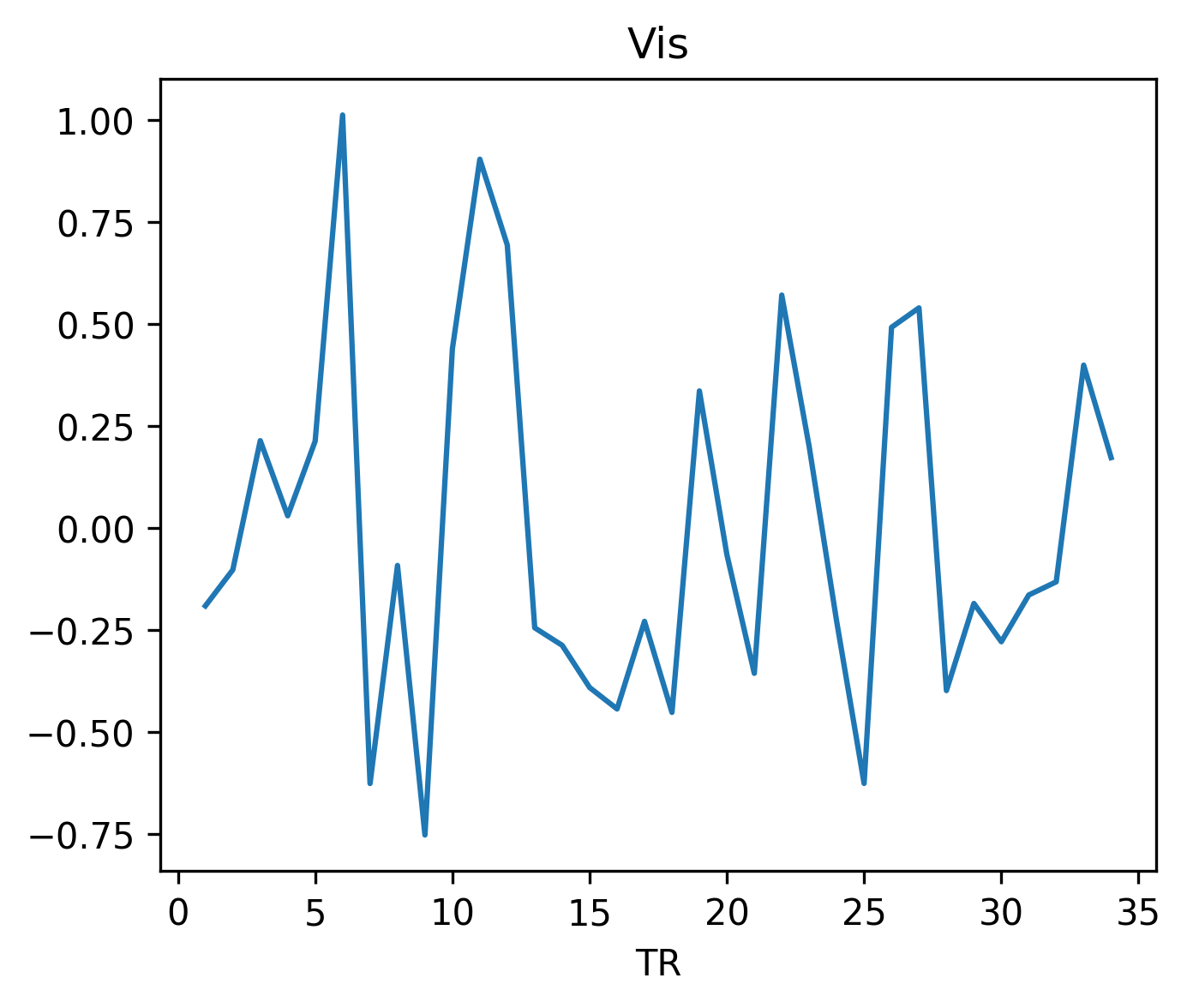
# Visualize BOLD Data
extractor.visualize_bold(subj_id="0004", run=1, region="Vis", figsize=(5, 4))
from neurocaps.analysis import CAP
# Initialize CAP class
cap_analysis = CAP(parcel_approach=extractor.parcel_approach)
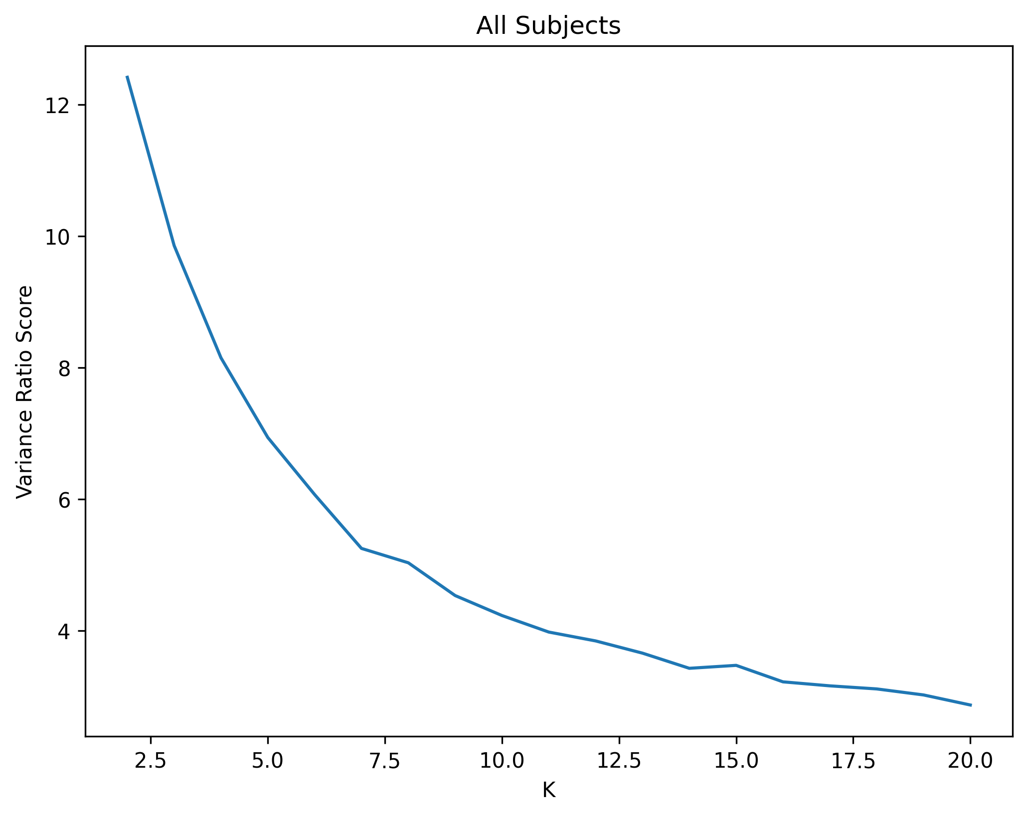
# Identify the optimal number of CAPs (clusters)
# using the variance_ratio method to test 2-10
# The optimal number of CAPs is automatically stored
cap_analysis.get_caps(
subject_timeseries=extractor.subject_timeseries,
n_clusters=range(2, 10),
standardize=True,
cluster_selection_method="variance_ratio",
max_iter=500,
n_init=10,
random_state=0,
show_figs=True,
)
2025-07-08 08:22:00,439 neurocaps.analysis.cap._internals.cluster [INFO] No groups specified. Using default group 'All Subjects' containing all subject IDs from `subject_timeseries`. The `groups` dictionary will remain fixed unless the `CAP` class is re-initialized or `clear_groups()` is used.
2025-07-08 08:22:01,315 neurocaps.analysis.cap._internals.cluster [INFO] [GROUP: All Subjects | METHOD: variance_ratio] Optimal cluster size is 2.
# Calculate temporal fraction and transition probability of each CAP for all subjects
output = cap_analysis.calculate_metrics(
    extractor.subject_timeseries, metrics=["temporal_fraction", "transition_probability"]
)
print(output["temporal_fraction"])
Subject_ID |
Group |
Run |
CAP-1 |
CAP-2 |
|---|---|---|---|---|
0004 |
All Subjects |
run-1 |
0.4117647058823529 |
0.5882352941176471 |
0004 |
All Subjects |
run-2 |
0.5 |
0.5 |
0006 |
All Subjects |
run-1 |
0.4864864864864865 |
0.5135135135135135 |
0006 |
All Subjects |
run-2 |
0.5161290322580645 |
0.4838709677419355 |
# Averaged transition probability matrix
from neurocaps.analysis import transition_matrix

transition_matrix(output["transition_probability"])

cap_analysis.caps2plot(plot_options="heatmap")

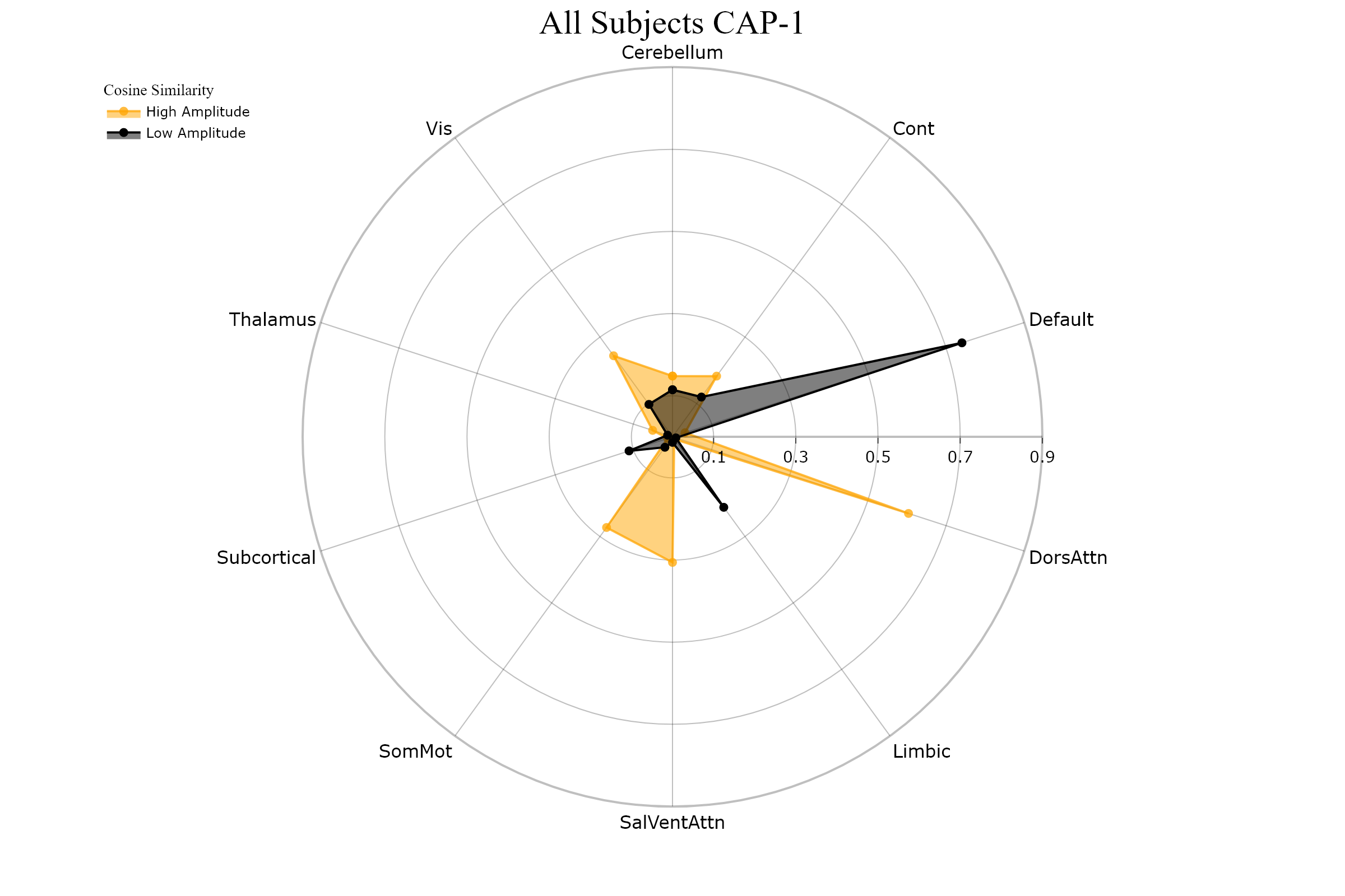
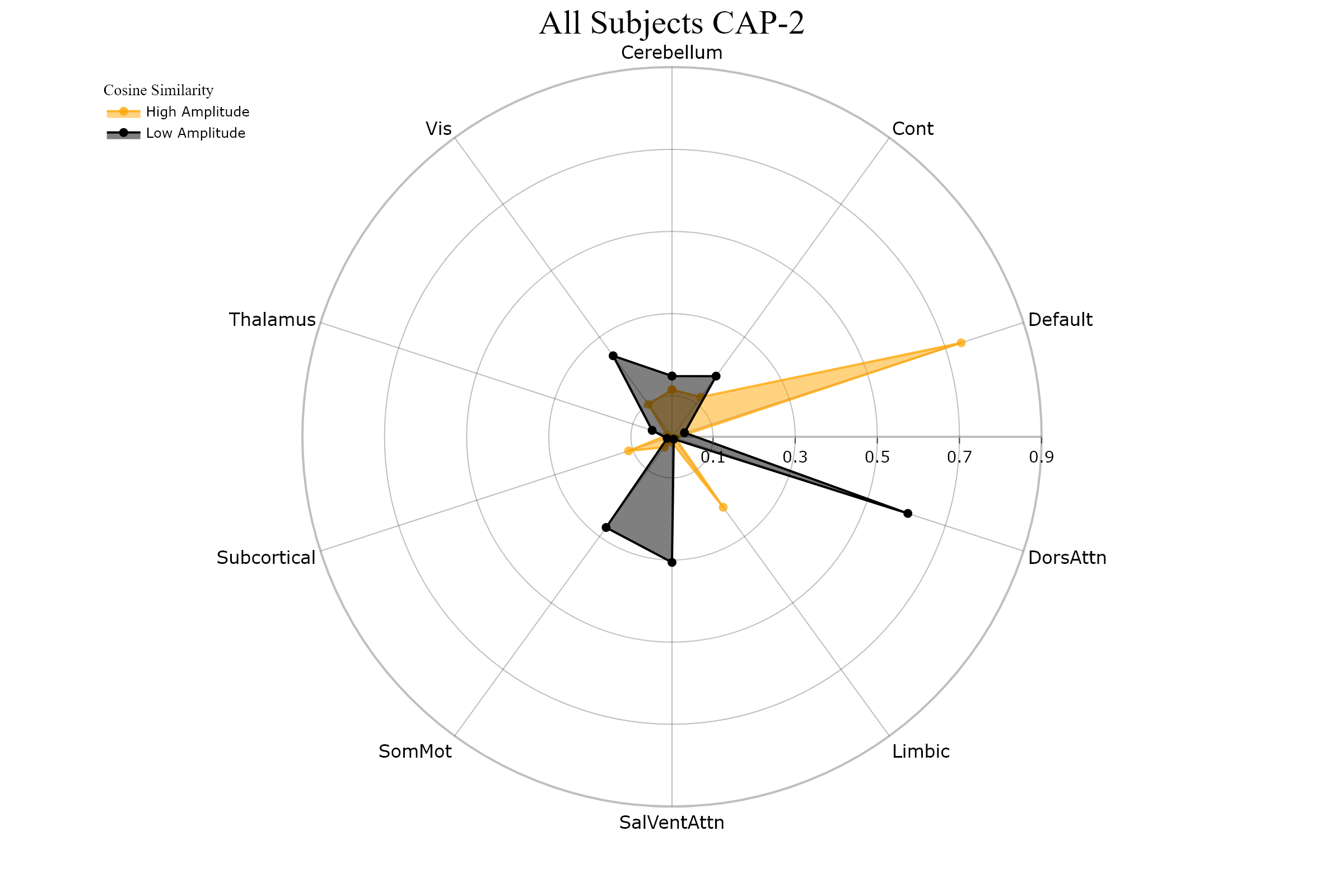
# Project CAPs onto surface plots
# and generate cosine similarity network alignment of CAPs

radialaxis = {
    "showline": True,
    "linewidth": 2,
    "linecolor": "rgba(0, 0, 0, 0.25)",
    "gridcolor": "rgba(0, 0, 0, 0.25)",
    "ticks": "outside",
    "tickfont": {"size": 14, "color": "black"},
    "range": [0, 0.5],
    "tickvals": [0.1, "", 0.3, "", 0.5],
}

color_discrete_map = {
    "High Amplitude": "rgba(255, 165, 0, 0.75)",
    "Low Amplitude": "black",
}

cap_analysis.caps2surf(color_range=(1, 1)).caps2radar(
    radialaxis=radialaxis, color_discrete_map=color_discrete_map
)